5 Ways To Create Dynamic Data Validation Lists In Excel

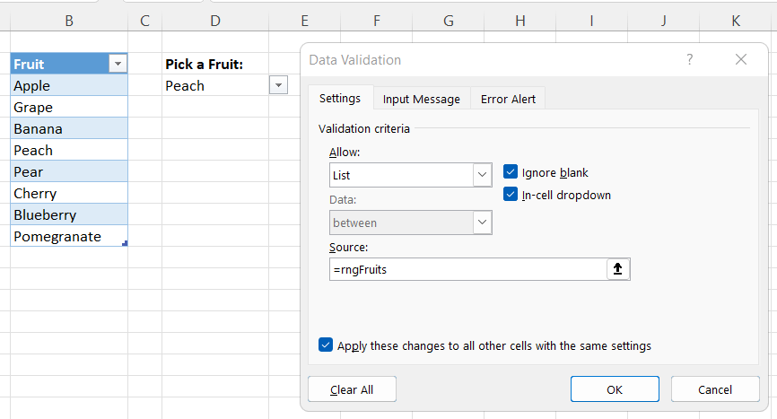
Data validation is a powerful feature in Excel that allows you to restrict the input of data in a cell or range of cells. One of the most useful applications of data validation is creating dynamic lists that update automatically based on the values in other cells or ranges. In this article, we will explore five ways to create dynamic data validation lists in Excel.

Dynamic data validation lists are essential in many real-world scenarios, such as creating drop-down menus that update based on user input, validating data against a list of approved values, or creating interactive dashboards that respond to changes in the data. By creating dynamic lists, you can make your Excel models more flexible, user-friendly, and efficient.

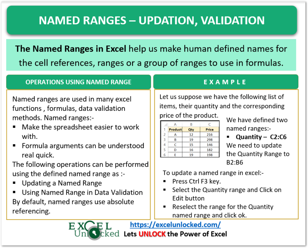
Method 1: Using Named Ranges and the Data Validation Feature

One of the simplest ways to create a dynamic data validation list is by using named ranges and the data validation feature. Here's how:

• Select the cell or range of cells where you want to create the dynamic list.
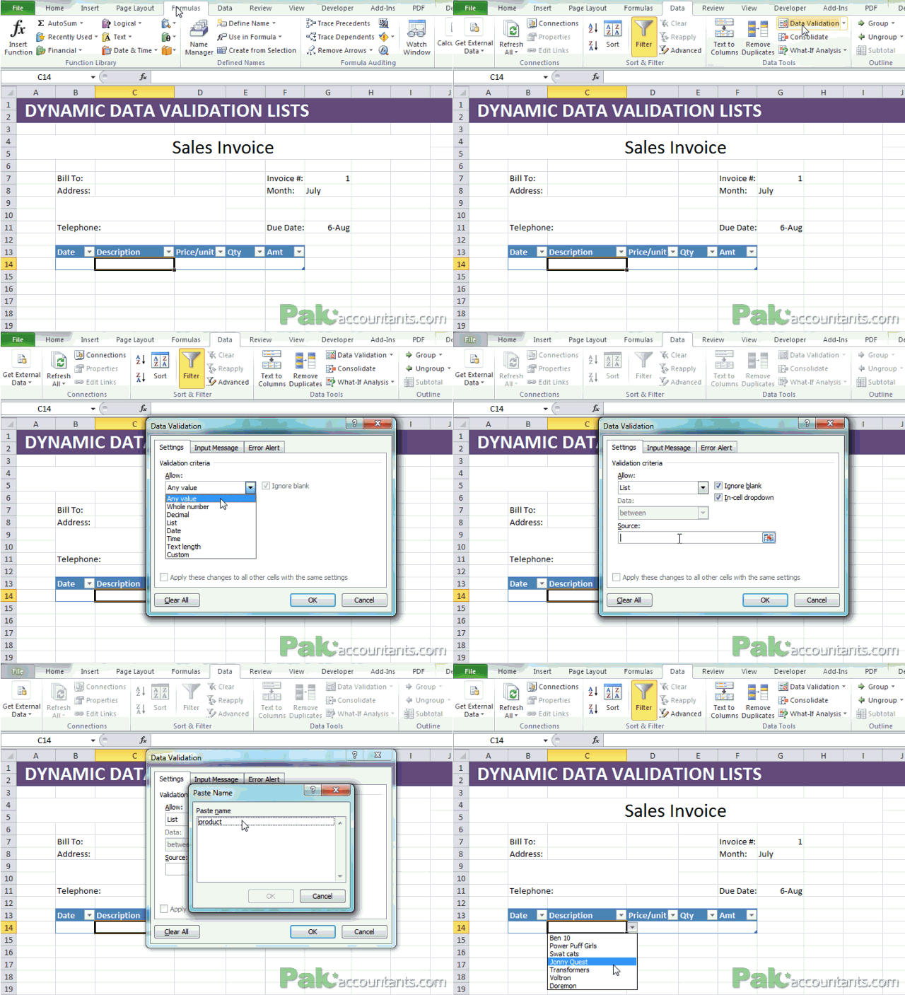
• Go to the "Data" tab in the ribbon and click on "Data Validation."
• In the "Data Validation" dialog box, select "List" from the "Allow" dropdown menu.
• In the "Source" field, enter the range of cells that contains the list of values you want to validate against.
• Click "OK" to apply the data validation.

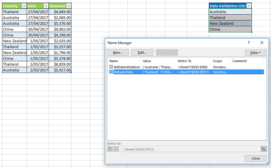
To make the list dynamic, you can use a named range to define the range of cells that contains the list of values. To create a named range, follow these steps:

• Select the range of cells that contains the list of values.
• Go to the "Formulas" tab in the ribbon and click on "Define Name."
• In the "New Name" dialog box, enter a name for the range, such as "ValidValues."
• Click "OK" to define the named range.

Once you've defined the named range, you can use it as the source for your data validation list. To do this, follow these steps:

• Select the cell or range of cells where you want to create the dynamic list.
• Go to the "Data" tab in the ribbon and click on "Data Validation."
• In the "Data Validation" dialog box, select "List" from the "Allow" dropdown menu.
• In the "Source" field, enter the name of the named range, such as "=ValidValues."
• Click "OK" to apply the data validation.

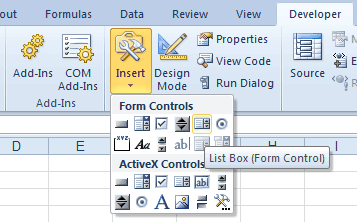
Method 2: Using the OFFSET and MATCH Functions

Another way to create a dynamic data validation list is by using the OFFSET and MATCH functions. Here's how:

• Select the cell or range of cells where you want to create the dynamic list.
• Go to the "Data" tab in the ribbon and click on "Data Validation."
• In the "Data Validation" dialog box, select "List" from the "Allow" dropdown menu.
• In the "Source" field, enter the following formula: =OFFSET($A$1,MATCH(TRUE,ISBLANK($A:$A),0)-1,0,COUNTA($A:$A)-MATCH(TRUE,ISBLANK($A:$A),0)+1)
• Click "OK" to apply the data validation.

This formula uses the OFFSET function to return a range of cells that starts at the first non-blank cell in column A and extends down to the last non-blank cell in column A. The MATCH function is used to find the first non-blank cell in column A, and the COUNTA function is used to count the number of non-blank cells in column A.

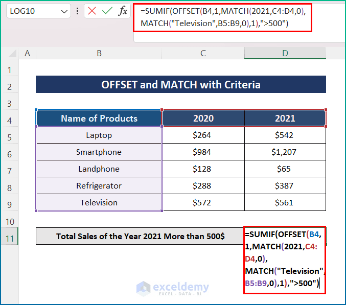
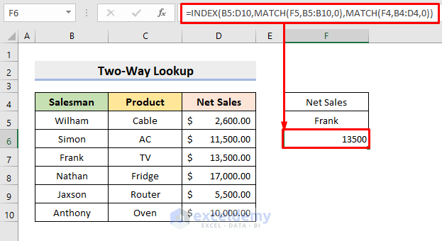
Method 3: Using the INDEX and MATCH Functions

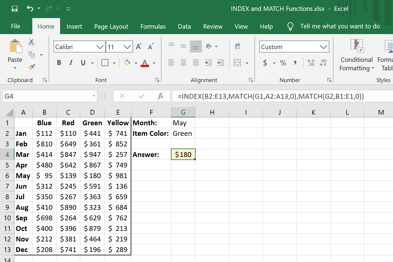
You can also use the INDEX and MATCH functions to create a dynamic data validation list. Here's how:

• Select the cell or range of cells where you want to create the dynamic list.
• Go to the "Data" tab in the ribbon and click on "Data Validation."
• In the "Data Validation" dialog box, select "List" from the "Allow" dropdown menu.
• In the "Source" field, enter the following formula: =INDEX($A:$A,MATCH(TRUE,ISBLANK($A:$A),0)):INDEX($A:$A,COUNTA($A:$A))
• Click "OK" to apply the data validation.

This formula uses the INDEX function to return a range of cells that starts at the first non-blank cell in column A and extends down to the last non-blank cell in column A. The MATCH function is used to find the first non-blank cell in column A, and the COUNTA function is used to count the number of non-blank cells in column A.

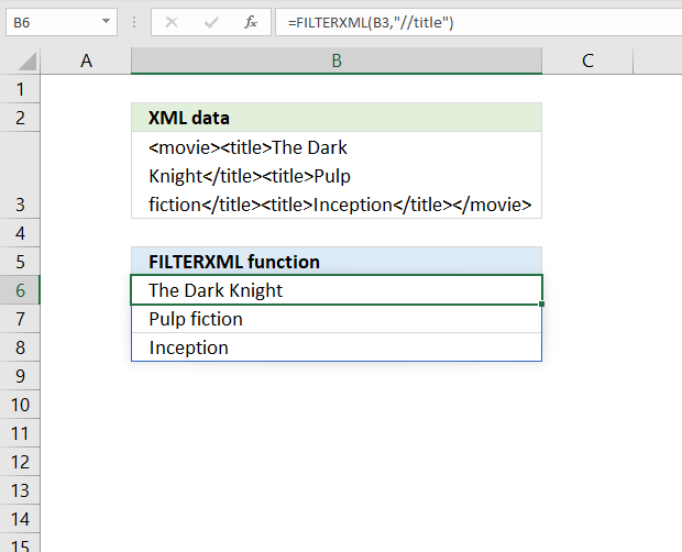
Method 4: Using the FILTERXML Function

If you're using Excel 2019 or later, you can use the FILTERXML function to create a dynamic data validation list. Here's how:

• Select the cell or range of cells where you want to create the dynamic list.
• Go to the "Data" tab in the ribbon and click on "Data Validation."
• In the "Data Validation" dialog box, select "List" from the "Allow" dropdown menu.
• In the "Source" field, enter the following formula: =FILTERXML("<t><d>"&TEXTJOIN("</d><d>",TRUE,$A:$A)&"</d></t>","//d")
• Click "OK" to apply the data validation.

This formula uses the FILTERXML function to parse the XML string and return a list of values. The TEXTJOIN function is used to concatenate the values in column A into a single string.

Method 5: Using Power Query

Finally, you can use Power Query to create a dynamic data validation list. Here's how:

• Select the cell or range of cells where you want to create the dynamic list.
• Go to the "Data" tab in the ribbon and click on "From Table/Range."
• In the "Create Table" dialog box, select the range of cells that contains the data you want to validate.
• Click "OK" to create the table.
• Go to the "Home" tab in the ribbon and click on "Edit Queries."
• In the "Query Editor" window, select the column that contains the list of values you want to validate.
• Go to the "Add Column" tab in the ribbon and click on "Custom Column."
• In the "Custom Column" dialog box, enter the following formula: =Table buffered
• Click "OK" to apply the formula.
• Go to the "Home" tab in the ribbon and click on "Load & Close."
• In the "Load To" dialog box, select the range of cells where you want to load the data.
• Click "OK" to load the data.

This formula uses Power Query to create a table that buffers the data in column A. The buffered data is then used to create a dynamic data validation list.