5 Ways To Use Multiple Criteria Vlookup In Excel

Excel's VLOOKUP function is an essential tool for data analysis and retrieval. However, its limitations become apparent when you need to search for data based on multiple criteria. Fortunately, Excel provides several ways to perform multiple criteria VLOOKUP, making it easier to work with complex data sets. In this article, we'll explore five ways to use multiple criteria VLOOKUP in Excel, helping you to take your data analysis skills to the next level.

Understanding Multiple Criteria VLOOKUP

Before diving into the different methods, it's essential to understand what multiple criteria VLOOKUP entails. In a standard VLOOKUP, you specify a single value to search for in a table array. However, when dealing with multiple criteria, you need to search for multiple values simultaneously, often in different columns. This requires a more advanced approach to retrieve the desired data.

Method 1: Using INDEX-MATCH Function

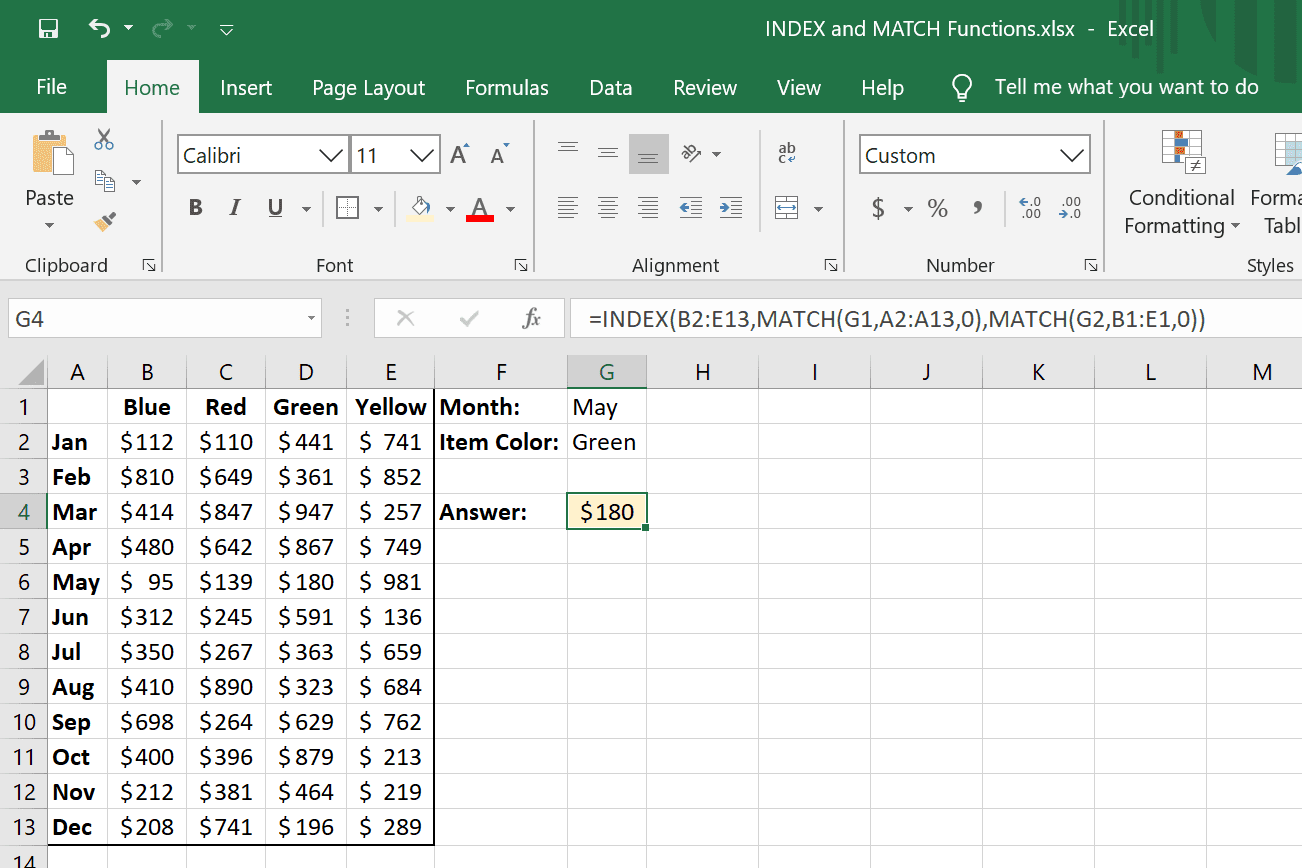
One of the most popular methods for multiple criteria VLOOKUP is using the INDEX-MATCH function combination. This approach is more flexible and powerful than the standard VLOOKUP.

To use INDEX-MATCH for multiple criteria VLOOKUP, follow these steps:

1. Select the cell where you want to display the result.
2. Use the MATCH function to search for the first criterion in the first column of the table array.
3. Use the MATCH function again to search for the second criterion in the second column of the table array.
4. Use the INDEX function to return the value at the intersection of the two matches.

Example:

=INDEX(C:C,MATCH(1,(A:A=A2)*(B:B=B2),0))

In this example, the formula searches for the value in cell A2 in column A and the value in cell B2 in column B. The INDEX function then returns the value in column C at the intersection of the two matches.

Method 2: Using VLOOKUP with Multiple Criteria using Helper Column

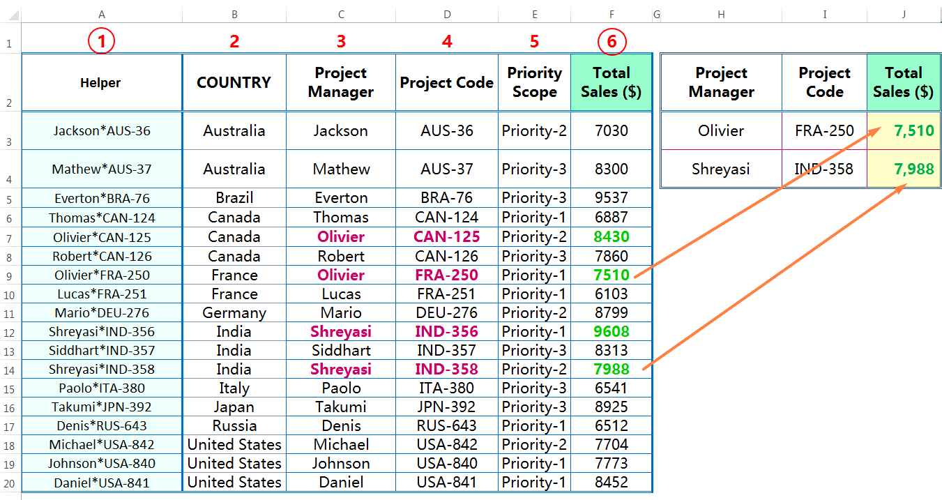
Another method for multiple criteria VLOOKUP involves creating a helper column that concatenates the multiple criteria. This approach is useful when you need to search for data based on multiple criteria in different columns.

To use VLOOKUP with a helper column, follow these steps:

1. Create a new column that concatenates the multiple criteria using the & operator.
2. Use the VLOOKUP function to search for the concatenated value in the helper column.
3. Return the value from the desired column.

Example:

=VLOOKUP(A2&B2,C:D,2,FALSE)

In this example, the formula concatenates the values in columns A and B using the & operator and searches for the result in the helper column. The VLOOKUP function then returns the value in column D.

Method 3: Using Power Query

Power Query is a powerful tool in Excel that allows you to manipulate and transform data. You can use Power Query to perform multiple criteria VLOOKUP by creating a new query that searches for data based on multiple criteria.

To use Power Query for multiple criteria VLOOKUP, follow these steps:

1. Go to the Data tab and select New Query.
2. Choose the table array as the data source.
3. Add a new column that searches for the multiple criteria using the & operator.
4. Return the desired value using the Return function.

Example:

=Return Table.SelectRows(#"Table", each ([ColumnA] = A2 and [ColumnB] = B2))

In this example, the formula creates a new query that searches for the values in columns A and B using the & operator. The Return function then returns the desired value.

Method 4: Using Multiple Criteria VLOOKUP with SUMIFS Function

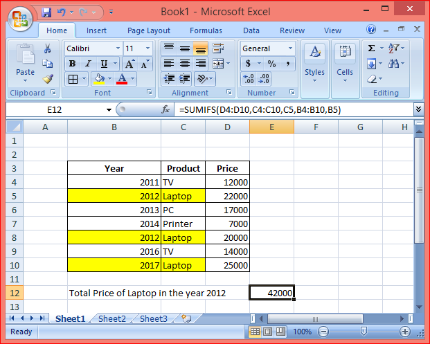
The SUMIFS function is a useful tool for summing values based on multiple criteria. You can also use the SUMIFS function to perform multiple criteria VLOOKUP by returning a single value instead of a sum.

To use the SUMIFS function for multiple criteria VLOOKUP, follow these steps:

1. Select the cell where you want to display the result.
2. Use the SUMIFS function to search for the multiple criteria.
3. Return the desired value using the Return function.

Example:

=SUMIFS(C:C,A:A,A2,B:B,B2)

In this example, the formula searches for the values in columns A and B using the SUMIFS function. The Return function then returns the desired value.

Method 5: Using Multiple Criteria VLOOKUP with FILTER Function

The FILTER function is a new function in Excel that allows you to filter data based on multiple criteria. You can use the FILTER function to perform multiple criteria VLOOKUP by returning a single value instead of a filtered range.

To use the FILTER function for multiple criteria VLOOKUP, follow these steps:

1. Select the cell where you want to display the result.
2. Use the FILTER function to search for the multiple criteria.
3. Return the desired value using the Return function.

Example:

=FILTER(C:C,(A:A=A2)*(B:B=B2))

In this example, the formula searches for the values in columns A and B using the FILTER function. The Return function then returns the desired value.

In conclusion, multiple criteria VLOOKUP is a powerful tool in Excel that allows you to search for data based on multiple criteria. The five methods outlined in this article provide different approaches to achieving this goal, from using the INDEX-MATCH function to the FILTER function. By mastering these methods, you can take your data analysis skills to the next level and make more informed decisions.