5 Ways To Use Isna In Excel

The ISNA function in Excel is a powerful tool that allows users to test if a cell contains a #N/A error. This function returns a TRUE or FALSE value, indicating whether the cell contains a #N/A error or not. In this article, we will explore five ways to use the ISNA function in Excel, along with practical examples and step-by-step instructions.

What is the ISNA Function in Excel?

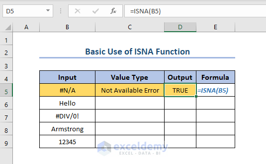
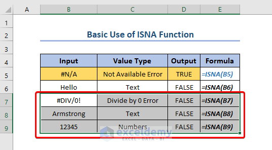
The ISNA function in Excel is a logical function that tests if a cell contains a #N/A error. The function returns a TRUE value if the cell contains a #N/A error, and a FALSE value if it does not. The syntax for the ISNA function is as follows:

ISNA(cell)

Where cell is the cell reference that you want to test for a #N/A error.

Method 1: Using ISNA to Test for #N/A Errors

One of the most common uses of the ISNA function is to test if a cell contains a #N/A error. This can be useful when working with formulas that may return a #N/A error, such as the VLOOKUP or INDEX/MATCH functions.

For example, suppose you have a formula that looks up a value in a table using the VLOOKUP function:

=VLOOKUP(A2, B:C, 2, FALSE)

If the value in cell A2 is not found in the table, the VLOOKUP function will return a #N/A error. To test if the formula returns a #N/A error, you can use the ISNA function:

=ISNA(VLOOKUP(A2, B:C, 2, FALSE))

If the formula returns a #N/A error, the ISNA function will return a TRUE value. Otherwise, it will return a FALSE value.

Method 2: Using ISNA with IF Statements

Another way to use the ISNA function is in combination with IF statements. This allows you to perform different actions based on whether a cell contains a #N/A error or not.

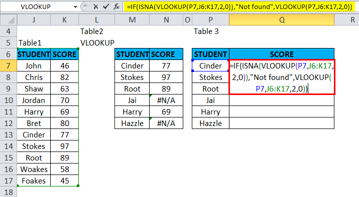
For example, suppose you want to display a custom error message if a formula returns a #N/A error. You can use the ISNA function with an IF statement to achieve this:

=IF(ISNA(VLOOKUP(A2, B:C, 2, FALSE)), "Error: Value not found", VLOOKUP(A2, B:C, 2, FALSE))

If the VLOOKUP function returns a #N/A error, the ISNA function will return a TRUE value, and the IF statement will display the custom error message. Otherwise, the IF statement will display the result of the VLOOKUP function.

Method 3: Using ISNA to Ignore #N/A Errors in Calculations

When performing calculations that involve cells that may contain #N/A errors, you can use the ISNA function to ignore these errors. This can be useful when working with formulas that involve multiple cells, some of which may contain #N/A errors.

For example, suppose you want to calculate the average of a range of cells that may contain #N/A errors. You can use the ISNA function to ignore these errors:

=AVERAGEIF(range, NOT(ISNA(range)))

This formula will calculate the average of the range, ignoring any cells that contain #N/A errors.

Method 4: Using ISNA to Count #N/A Errors

You can also use the ISNA function to count the number of cells in a range that contain #N/A errors. This can be useful when troubleshooting formulas or data.

For example, suppose you want to count the number of cells in a range that contain #N/A errors:

=COUNTIF(range, ISNA(range))

This formula will return the number of cells in the range that contain #N/A errors.

Method 5: Using ISNA with Array Formulas

Finally, you can use the ISNA function with array formulas to perform complex calculations that involve multiple cells and #N/A errors.

For example, suppose you want to calculate the sum of a range of cells that may contain #N/A errors, and you want to ignore these errors. You can use the ISNA function with an array formula to achieve this:

=SUM(IF(ISNA(range), 0, range))

This formula will calculate the sum of the range, ignoring any cells that contain #N/A errors.

Gallery of ISNA Function Examples

Frequently Asked Questions

Conclusion

The ISNA function in Excel is a powerful tool that allows users to test if a cell contains a #N/A error. By using the ISNA function in combination with IF statements, to ignore #N/A errors in calculations, to count #N/A errors, and with array formulas, you can create complex formulas and calculations that handle #N/A errors with ease. We hope this article has helped you to understand how to use the ISNA function in Excel, and we encourage you to try out the examples and methods outlined in this article.

Gallery of 5 Ways To Use Isna In Excel