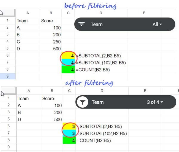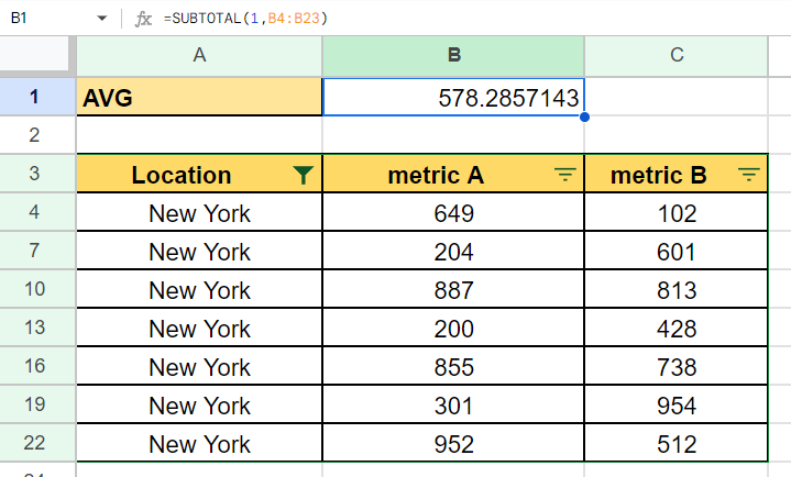
Google Sheets is a powerful tool that offers a wide range of functions to help users manage and analyze data. One of the most useful functions in Google Sheets is the SUBTOTAL function, which allows users to calculate subtotals and totals for a specific range of cells. In this article, we will explore five ways to use the SUBTOTAL function in Google Sheets.
The SUBTOTAL function is particularly useful when working with large datasets, as it allows users to easily calculate subtotals and totals without having to manually create formulas. This function is also dynamic, meaning that it will automatically update when changes are made to the data range.
What is the SUBTOTAL Function?
The SUBTOTAL function in Google Sheets is a mathematical function that calculates the subtotal of a specific range of cells. The function uses the following syntax:
SUBTOTAL(function_num, range1, [range2,...])
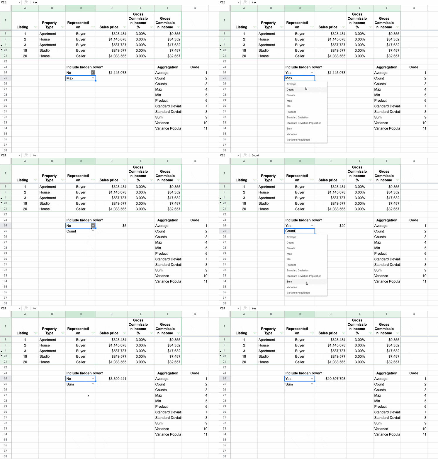
- function_num: This is the number of the function to be applied to the range. For example, 1 for AVERAGE, 2 for COUNT, 3 for COUNTA, and so on.
- range1: This is the range of cells that you want to calculate the subtotal for.
- range2: This is an optional range of cells that you can include in the calculation.
5 Ways to Use the SUBTOTAL Function
1. Calculating Subtotals for a Range of Cells
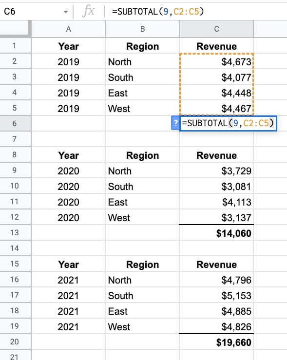
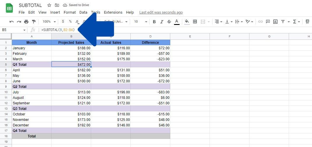
One of the most common uses of the SUBTOTAL function is to calculate subtotals for a range of cells. For example, let's say you have a list of sales data for different regions, and you want to calculate the subtotal for each region.

To calculate the subtotal for each region, you can use the following formula:
=SUBTOTAL(9, B2:B10)
In this formula, 9 is the function number for SUM, and B2:B10 is the range of cells that you want to calculate the subtotal for.
2. Calculating Subtotals for Multiple Ranges
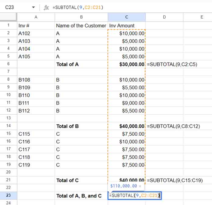
The SUBTOTAL function can also be used to calculate subtotals for multiple ranges of cells. For example, let's say you have two lists of sales data for different regions, and you want to calculate the subtotal for each region.

To calculate the subtotal for each region, you can use the following formula:
=SUBTOTAL(9, B2:B10, D2:D10)
In this formula, 9 is the function number for SUM, B2:B10 is the first range of cells, and D2:D10 is the second range of cells.
3. Calculating Subtotals with Multiple Criteria
The SUBTOTAL function can also be used to calculate subtotals with multiple criteria. For example, let's say you have a list of sales data for different regions and products, and you want to calculate the subtotal for each region and product.

To calculate the subtotal for each region and product, you can use the following formula:
=SUBTOTAL(9, B2:B10, C2:C10)
In this formula, 9 is the function number for SUM, B2:B10 is the first range of cells, and C2:C10 is the second range of cells.
4. Calculating Subtotals with Errors
The SUBTOTAL function can also be used to calculate subtotals with errors. For example, let's say you have a list of sales data for different regions, and you want to calculate the subtotal for each region, but some of the cells contain errors.

To calculate the subtotal for each region, ignoring the errors, you can use the following formula:
=SUBTOTAL(9, B2:B10, IF(ISERROR(B2:B10), "", B2:B10))
In this formula, 9 is the function number for SUM, B2:B10 is the range of cells, and IF(ISERROR(B2:B10), "", B2:B10) is the range of cells with errors ignored.
5. Calculating Subtotals with Conditional Formatting
The SUBTOTAL function can also be used to calculate subtotals with conditional formatting. For example, let's say you have a list of sales data for different regions, and you want to calculate the subtotal for each region, but only for the cells that meet a certain condition.

To calculate the subtotal for each region, you can use the following formula:
=SUBTOTAL(9, B2:B10, IF(C2:C10>100, B2:B10, ""))
In this formula, 9 is the function number for SUM, B2:B10 is the range of cells, and IF(C2:C10>100, B2:B10, "") is the range of cells with the condition applied.
Gallery of Google Sheets Subtotal Function Examples


Frequently Asked Questions
What is the SUBTOTAL function in Google Sheets?
+The SUBTOTAL function is a mathematical function in Google Sheets that calculates the subtotal of a specific range of cells.
How do I use the SUBTOTAL function in Google Sheets?
+To use the SUBTOTAL function, you need to specify the function number, range of cells, and optional range of cells. For example, =SUBTOTAL(9, B2:B10) calculates the subtotal of the range B2:B10.
Can I use the SUBTOTAL function with multiple ranges?
+Yes, you can use the SUBTOTAL function with multiple ranges by separating the ranges with commas. For example, =SUBTOTAL(9, B2:B10, D2:D10) calculates the subtotal of the ranges B2:B10 and D2:D10.
In conclusion, the SUBTOTAL function is a powerful tool in Google Sheets that allows users to calculate subtotals and totals for specific ranges of cells. With its flexibility and dynamic nature, this function can be used in a variety of scenarios, from simple calculations to complex data analysis. By following the examples and guidelines provided in this article, you can unlock the full potential of the SUBTOTAL function and take your data analysis to the next level.
