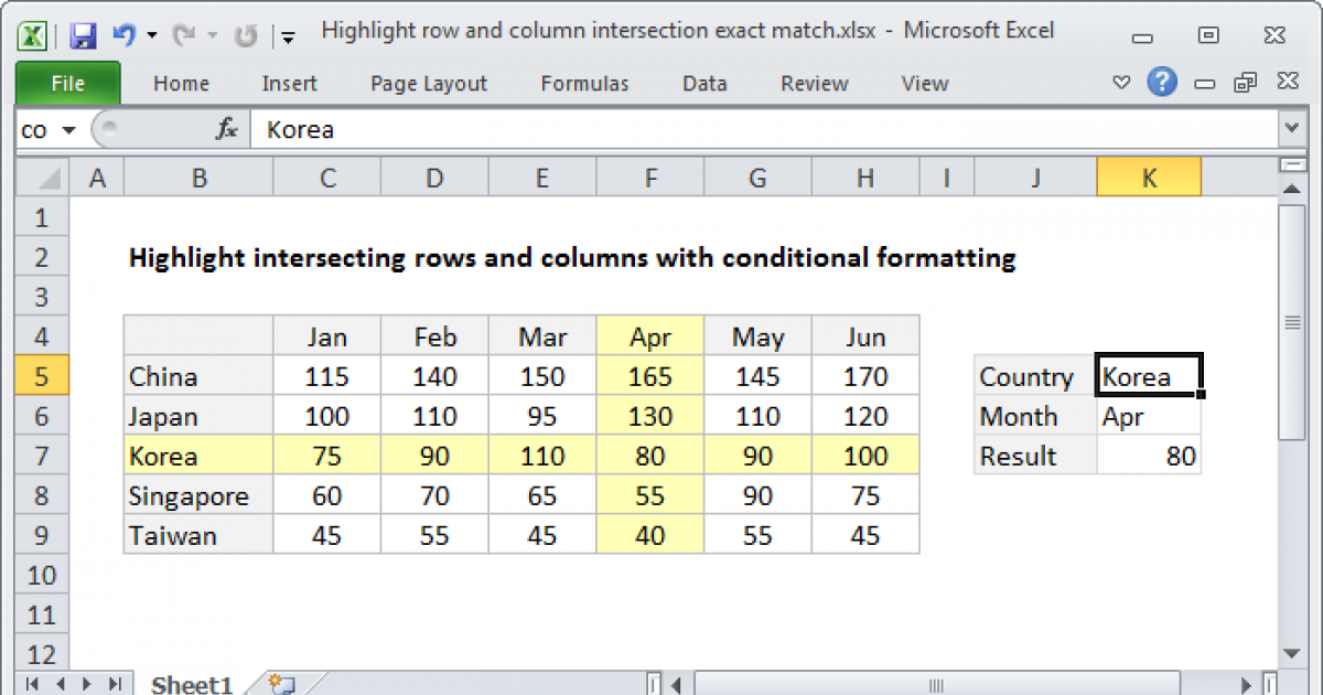
5 Ways To Highlight Matching Values In Excel

Highlighting matching values in Excel is an essential skill for data analysts, accountants, and anyone who works with large datasets. It helps to identify trends, patterns, and discrepancies in the data, making it easier to make informed decisions. In this article, we will explore five ways to highlight matching values in Excel.

Highlighting matching values is a powerful feature in Excel that can save you time and effort when working with large datasets. It allows you to quickly identify cells that contain the same value, making it easier to analyze and understand your data. Whether you're working with numbers, text, or dates, highlighting matching values is an essential skill to master.

In this article, we will explore five ways to highlight matching values in Excel. From using the built-in formatting tools to creating custom formulas, we will cover the most effective methods to highlight matching values in your spreadsheet.

Method 1: Using Conditional Formatting

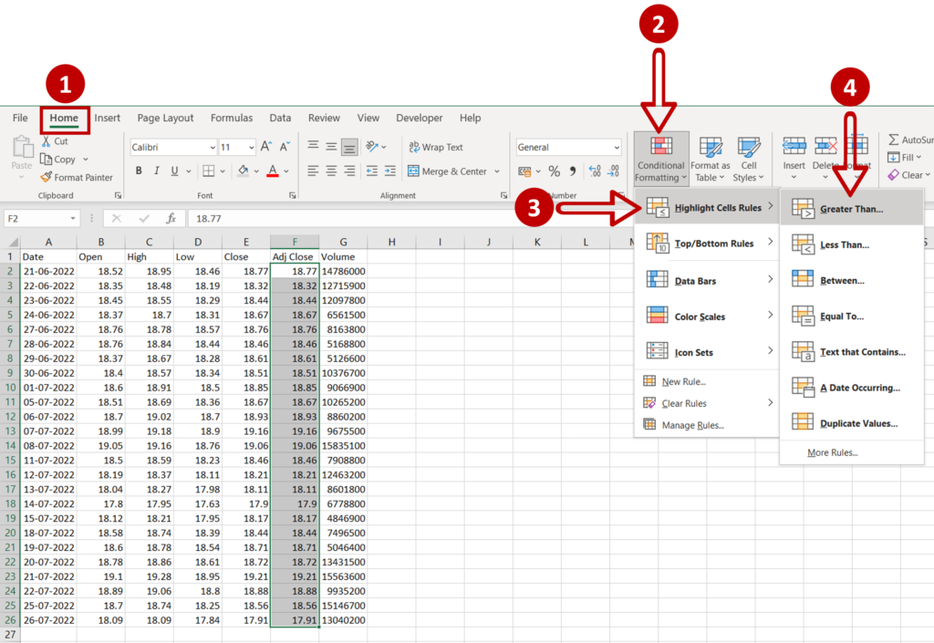
Conditional formatting is a powerful feature in Excel that allows you to highlight cells based on specific conditions. To highlight matching values using conditional formatting, follow these steps:

Select the range of cells that you want to format.
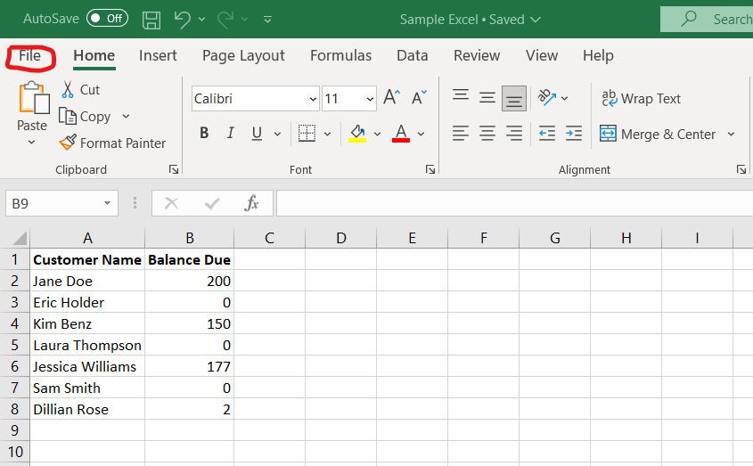
Go to the "Home" tab in the Excel ribbon.
Click on the "Conditional Formatting" button in the "Styles" group.
Select "Highlight Cells Rules" from the drop-down menu.
Choose "Duplicate Values" from the list of options.
Select the formatting style that you want to apply to the matching values.

Using conditional formatting is a quick and easy way to highlight matching values in Excel. It's a great method to use when you need to identify duplicate values in a range of cells.

Method 2: Using Formulas

You can also use formulas to highlight matching values in Excel. One way to do this is by using the COUNTIF function. Here's an example:

Select the range of cells that you want to format.
Enter the following formula in a new column: =COUNTIF(range, cell_value)>1
Replace "range" with the range of cells that you want to check for duplicates.
Replace "cell_value" with the value in the cell that you want to check.
If the formula returns a value greater than 1, it means that the value is a duplicate.

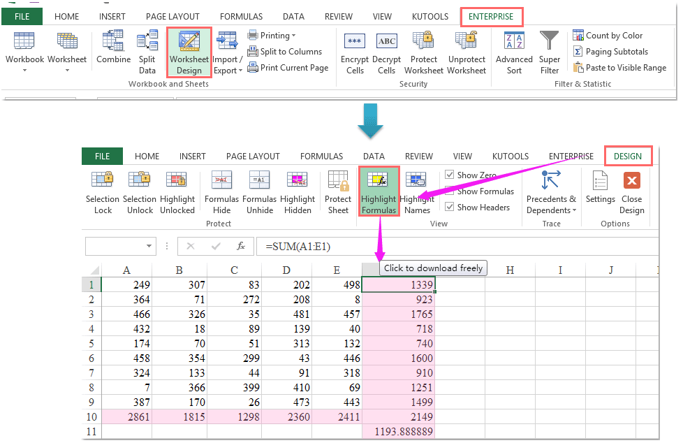
You can then use the formula to highlight the matching values by using conditional formatting. Simply select the range of cells that you want to format, go to the "Home" tab, and click on the "Conditional Formatting" button. Choose "New Rule" from the drop-down menu, and then select "Use a formula to determine which cells to format." Enter the formula that you created earlier, and then select the formatting style that you want to apply.

Method 3: Using VLOOKUP

VLOOKUP is a powerful function in Excel that allows you to look up values in a table and return a corresponding value from another column. You can use VLOOKUP to highlight matching values by creating a formula that checks for duplicates.

Here's an example:

Select the range of cells that you want to format.
Enter the following formula in a new column: =VLOOKUP(cell_value, range, 2, FALSE)>1
Replace "cell_value" with the value in the cell that you want to check.
Replace "range" with the range of cells that you want to check for duplicates.
If the formula returns a value greater than 1, it means that the value is a duplicate.

Method 4: Using Power Query

Power Query is a powerful tool in Excel that allows you to create custom queries to manipulate and analyze your data. You can use Power Query to highlight matching values by creating a custom query that checks for duplicates.

Here's an example:

Select the range of cells that you want to format.
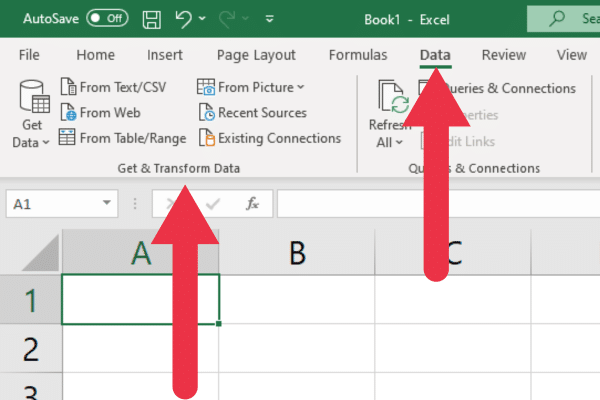
Go to the "Data" tab in the Excel ribbon.
Click on the "New Query" button in the "Get & Transform Data" group.
Select "From Table/Range" from the drop-down menu.
Choose the range of cells that you want to check for duplicates.
Click on the "OK" button to create the query.

Once you've created the query, you can use the "Group By" feature to check for duplicates. Simply click on the "Group By" button in the "Home" tab, and then select the column that you want to check for duplicates. If you find any duplicates, you can then use conditional formatting to highlight the matching values.

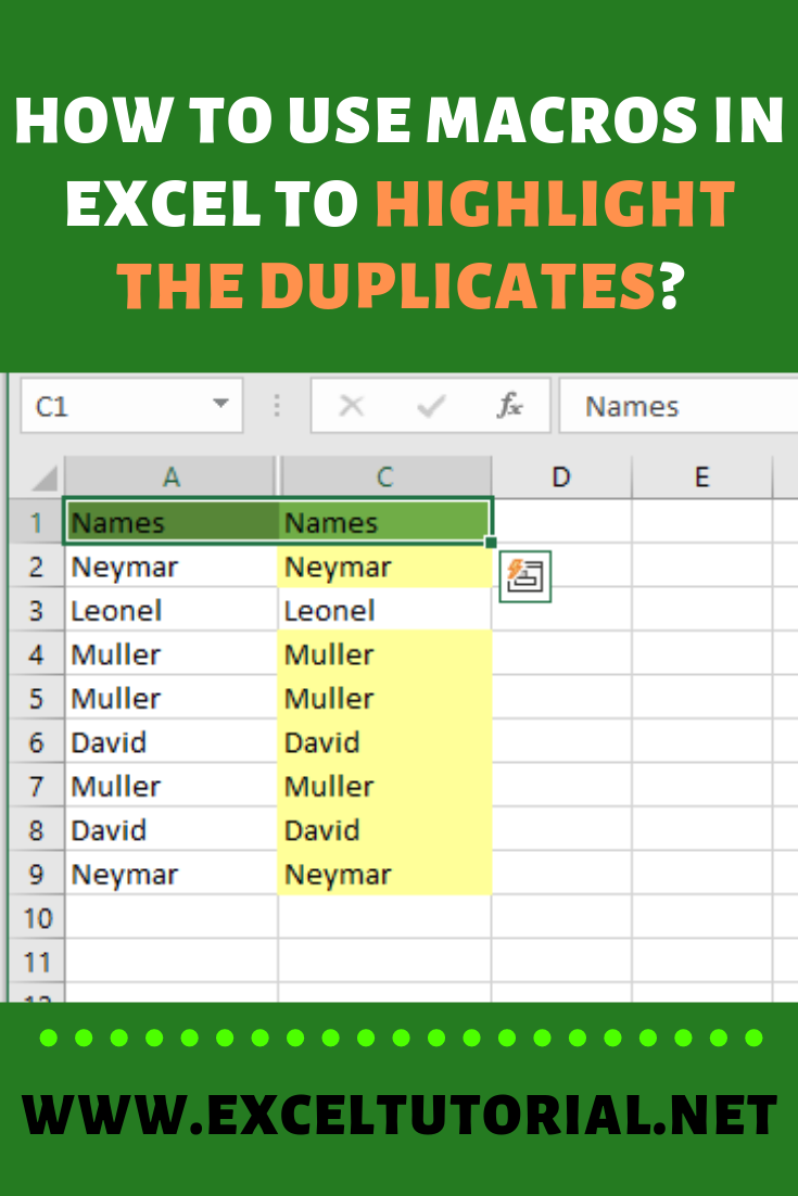
Method 5: Using Macros

Macros are a powerful feature in Excel that allows you to automate repetitive tasks. You can use macros to highlight matching values by creating a custom script that checks for duplicates.

Here's an example:

Select the range of cells that you want to format.
Go to the "Developer" tab in the Excel ribbon.
Click on the "Visual Basic" button in the "Code" group.
In the Visual Basic Editor, click on the "Insert" menu and select "Module."
Paste the following code into the module:

Sub HighlightDuplicates()
    Dim cell As Range
    For Each cell In Selection
        If cell.Value <> "" Then
            If Application.WorksheetFunction.CountIf(Range("A:A"), cell.Value) > 1 Then
                cell.Interior.ColorIndex = 6
            End If
        End If
    Next cell
End Sub

This code will highlight any cells that contain duplicate values in the range that you selected. Simply run the macro by clicking on the "Run" button in the Visual Basic Editor.

Conclusion

Highlighting matching values in Excel is a powerful feature that can save you time and effort when working with large datasets. Whether you're using conditional formatting, formulas, VLOOKUP, Power Query, or macros, there are many ways to highlight matching values in Excel. By mastering these techniques, you can become more efficient and effective in your work, and make better decisions with your data.

We hope this article has been helpful in teaching you how to highlight matching values in Excel. If you have any questions or need further assistance, please don't hesitate to ask.

What is the best way to highlight matching values in Excel?

The best way to highlight matching values in Excel depends on the specific needs of your project. You can use conditional formatting, formulas, VLOOKUP, Power Query, or macros to highlight matching values.

How do I use conditional formatting to highlight matching values in Excel?

To use conditional formatting to highlight matching values in Excel, select the range of cells that you want to format, go to the "Home" tab, and click on the "Conditional Formatting" button. Choose "Highlight Cells Rules" from the drop-down menu, and then select "Duplicate Values" from the list of options.