Excel is a powerful tool for data analysis, and mastering its various functions can significantly improve your productivity. Two of the most versatile and widely used functions in Excel are INDEX and MATCH. While often used separately, combining these functions can help you tackle complex data challenges, especially when dealing with multiple columns. This article will delve into the details of how to use Excel's INDEX-MATCH function with multiple columns, providing you with practical examples and steps to enhance your data analysis capabilities.
Understanding INDEX and MATCH Functions
Before diving into using INDEX-MATCH with multiple columns, it's essential to grasp what each function does individually.
-
INDEX Function: The INDEX function returns a value or the reference of the value at the intersection of a particular row and column. It can be used to look up values within a table or range by specifying the row and column numbers.
-
MATCH Function: The MATCH function searches for a specified item in a range of cells, then returns the relative position of that item in the range. This function is crucial for finding the position of a value in a range, which can then be used by the INDEX function.
Combining INDEX and MATCH for Multiple Columns
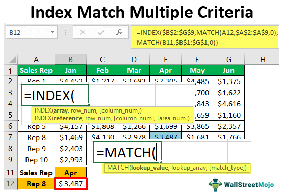
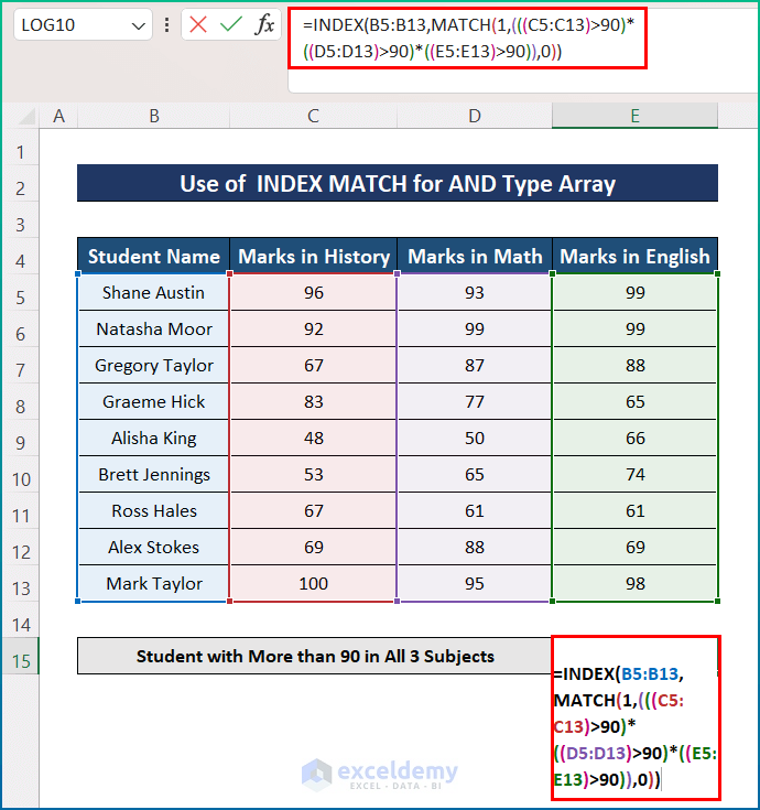
When working with multiple columns, you often need to look up a value based on more than one criterion. This is where combining the INDEX and MATCH functions becomes incredibly useful. The basic syntax for using INDEX-MATCH with multiple columns is as follows:
INDEX(range, MATCH(1, (condition1) * (condition2) *..., 0))
Where:
rangeis the range of cells from which you want to return a value.condition1,condition2, etc., are the conditions based on which you are looking up the value. These conditions are typically formulated using the MATCH function, which searches for specific values in different columns.- The multiplication of conditions creates an array of 1s and 0s that the outer MATCH function can then process to find the correct position.
Practical Examples
Let's consider some practical examples to illustrate how to use the INDEX-MATCH function with multiple columns.
Example 1: Finding a Specific Value Based on Two Conditions
Suppose you have a table with student names in Column A, their grades in Column B, and their attendance in Column C. You want to find the attendance of a student who has a specific name and grade.
| Student Name | Grade | Attendance |
|---|---|---|
| John | A | 95 |
| Jane | B | 90 |
| John | B | 92 |
| Jane | A | 98 |
To find the attendance of John with an A grade, you can use the following formula:
=INDEX(C:C, MATCH(1, (A:A="John") * (B:B="A"), 0))
This formula looks up the value "John" in Column A and "A" in Column B, and then returns the corresponding attendance value from Column C.
Example 2: Using INDEX-MATCH with Multiple Criteria Across Different Columns
Imagine you're working with a dataset of employees, including their department, job title, and salary. You need to find the salary of an employee based on their department and job title.
| Department | Job Title | Salary |
|---|---|---|
| Sales | Manager | 60000 |
| Marketing | Manager | 70000 |
| Sales | Analyst | 40000 |
| Marketing | Analyst | 45000 |
To find the salary of a Manager in the Sales department, you would use:
=INDEX(C:C, MATCH(1, (A:A="Sales") * (B:B="Manager"), 0))
This formula searches for "Sales" in Column A and "Manager" in Column B, and then returns the salary from Column C.
Tips for Using INDEX-MATCH with Multiple Columns
-
Use Absolute References: When using the INDEX-MATCH function, especially with multiple columns, it's advisable to use absolute references (e.g.,
$A$2) for the range and criteria ranges to ensure the formula doesn't shift when copied or moved. -
Manage Array Formulas: The multiplication of conditions within the MATCH function creates an array formula. Be cautious with array formulas, as they can slow down your spreadsheet, especially with large datasets.
-
Troubleshooting: If your formula doesn't return the expected result, check the criteria ranges and ensure they match the values you're looking for. Also, verify that the range specified in the INDEX function contains the values you want to return.

Gallery of Excel INDEX-MATCH Functions


FAQs
What is the advantage of using INDEX-MATCH over VLOOKUP in Excel?
+INDEX-MATCH offers more flexibility and power than VLOOKUP, especially when dealing with multiple criteria or looking up values to the left. It also allows for more dynamic range references.
Can I use INDEX-MATCH with more than two conditions?
+Yes, you can extend the INDEX-MATCH function to handle more than two conditions by multiplying additional criteria in the MATCH function.
How do I troubleshoot if my INDEX-MATCH formula isn't working?
+Check that your criteria ranges are correctly referenced and that the values you're looking for match exactly. Also, ensure the formula is entered correctly, including the use of absolute references if necessary.
In conclusion, mastering the use of the INDEX-MATCH function with multiple columns in Excel can significantly enhance your data analysis capabilities. Whether you're looking to find specific values based on multiple criteria or simplify complex lookups, this function combination is a powerful tool in your Excel arsenal. Practice makes perfect, so don't hesitate to experiment and apply these techniques to your own data challenges.


