5 Ways To Compare Strings In Excel

Comparing strings in Excel is a common task that can be accomplished using various formulas and techniques. Whether you're trying to identify duplicates, differences, or similarities between two sets of text data, Excel provides a range of tools to help you achieve your goals. In this article, we'll explore five ways to compare strings in Excel, including using formulas, functions, and conditional formatting.

Why Compare Strings in Excel?

Comparing strings in Excel is useful in a variety of situations, such as:

• Data cleaning and validation: Comparing strings can help you identify and correct errors or inconsistencies in your data.
• Data analysis: By comparing strings, you can identify patterns and trends in your data, such as common phrases or keywords.
• Data matching: Comparing strings can help you match data between different lists or tables, such as identifying duplicate records.

Method 1: Using the EXACT Function

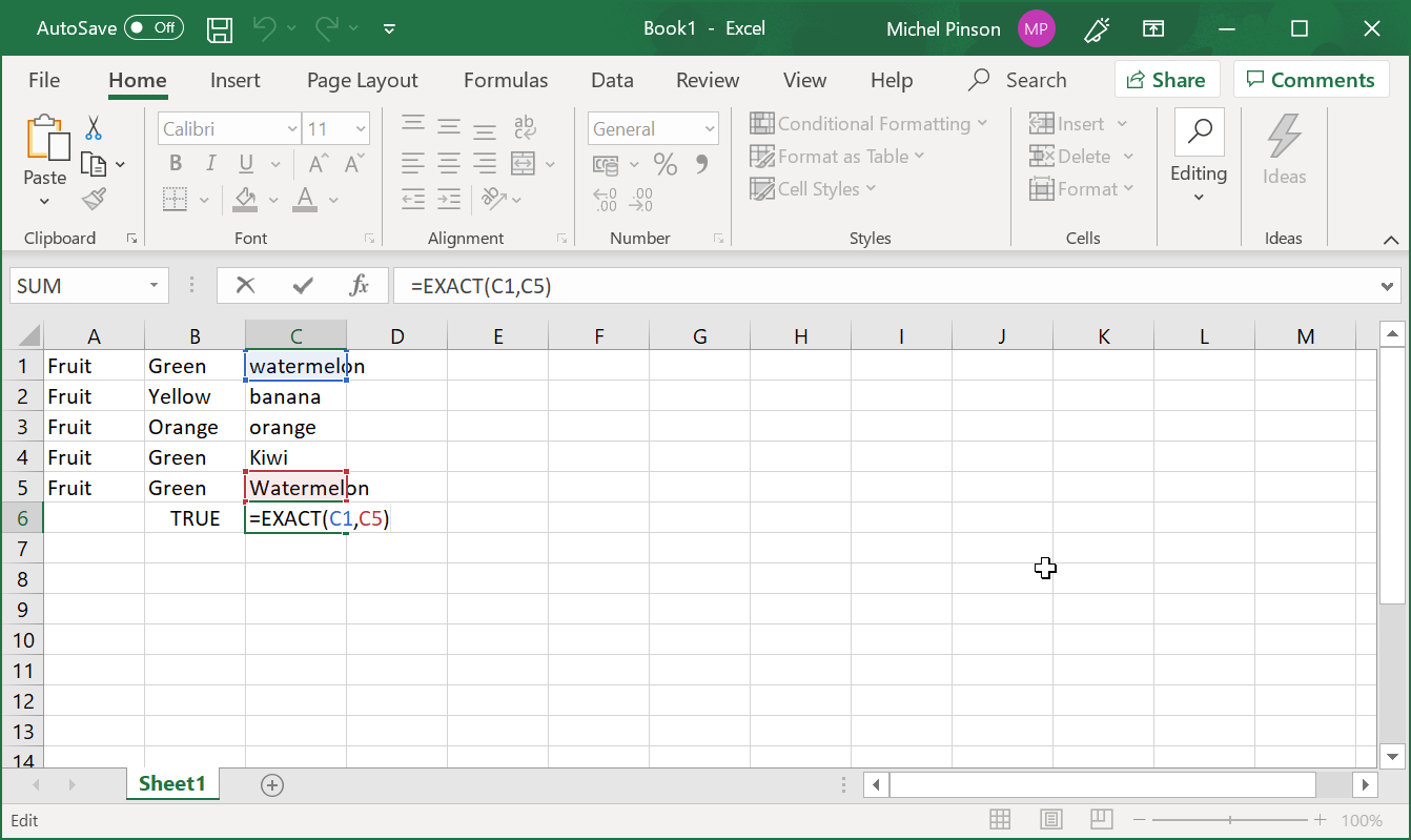
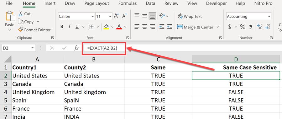
The EXACT function is a simple and straightforward way to compare two strings in Excel. This function returns TRUE if the two strings are identical, and FALSE otherwise.

Syntax: EXACT(text1, text2)

Example: =EXACT(A1, B1)

This formula compares the values in cells A1 and B1. If the values are identical, the formula returns TRUE. Otherwise, it returns FALSE.

Method 2: Using the IF and EXACT Functions

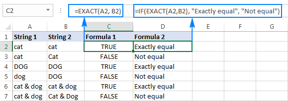
You can use the IF function in combination with the EXACT function to compare two strings and return a custom result.

Syntax: IF(EXACT(text1, text2), [result_if_true], [result_if_false])

Example: =IF(EXACT(A1, B1), "Match", "No Match")

This formula compares the values in cells A1 and B1. If the values are identical, the formula returns "Match". Otherwise, it returns "No Match".

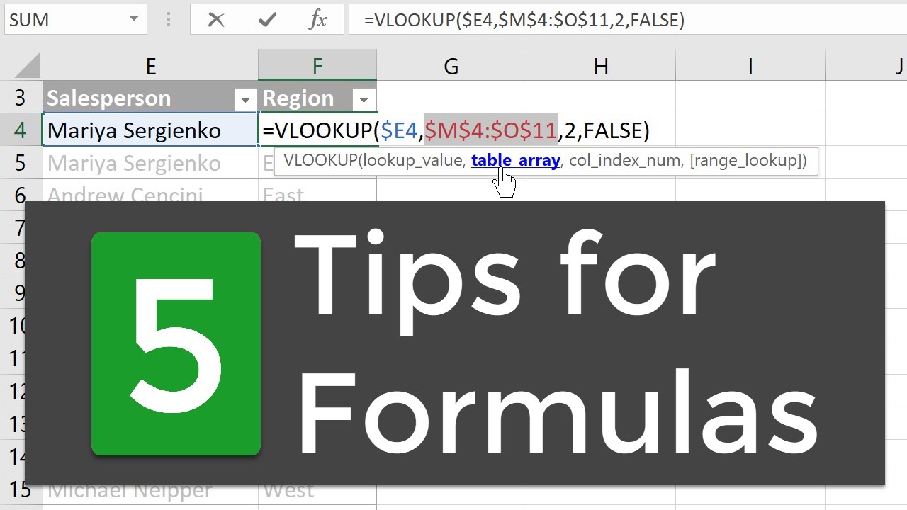
Method 3: Using the VLOOKUP Function

The VLOOKUP function can be used to compare a string value in one column with a range of values in another column.

Syntax: VLOOKUP(lookup_value, table_array, col_index_num, [range_lookup])

Example: =VLOOKUP(A1, B:C, 2, FALSE)

This formula looks up the value in cell A1 in the first column of the range B:C. If a match is found, the formula returns the corresponding value in the second column.

Method 4: Using Conditional Formatting

Conditional formatting can be used to compare strings and highlight differences or similarities.

Example:

1. Select the range of cells you want to compare.
2. Go to the Home tab in the Excel ribbon.
3. Click on the Conditional Formatting button.
4. Select "Highlight Cells Rules" > "Duplicate Values".
5. Choose the formatting options you want to apply.

This will highlight any duplicate values in the selected range.

Method 5: Using Power Query

Power Query is a powerful tool in Excel that allows you to compare and transform data.

Example:

1. Go to the Data tab in the Excel ribbon.
2. Click on the "From Other Sources" button.
3. Select "Blank Query".
4. In the Query Editor, click on the "Add Column" button.
5. Select "Custom Column".
6. Enter the following formula: =EXACT([Column1], [Column2])

This will create a new column that compares the values in the two selected columns.

We hope this article has provided you with a comprehensive overview of the different ways to compare strings in Excel. Whether you're a beginner or an advanced user, these methods can help you to analyze and transform your data with ease.

If you have any questions or need further assistance, please don't hesitate to comment below.

Gallery of 5 Ways To Compare Strings In Excel