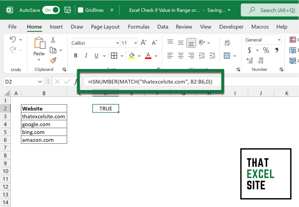
Determining true or false values in Excel can be a powerful way to analyze and manipulate data. One of the most effective ways to achieve this is by using the MATCH function in combination with other functions. In this article, we will explore five ways to use the MATCH function in Excel to determine true or false values.
The MATCH function is a lookup function that returns the position of a value within a range or array. By combining the MATCH function with other functions, such as the IF and ISNUMBER functions, you can create powerful formulas that determine true or false values based on specific conditions.
Method 1: Using MATCH with IF Function
One of the simplest ways to use the MATCH function to determine true or false values is by combining it with the IF function. The IF function checks if a condition is true or false and returns a value accordingly.
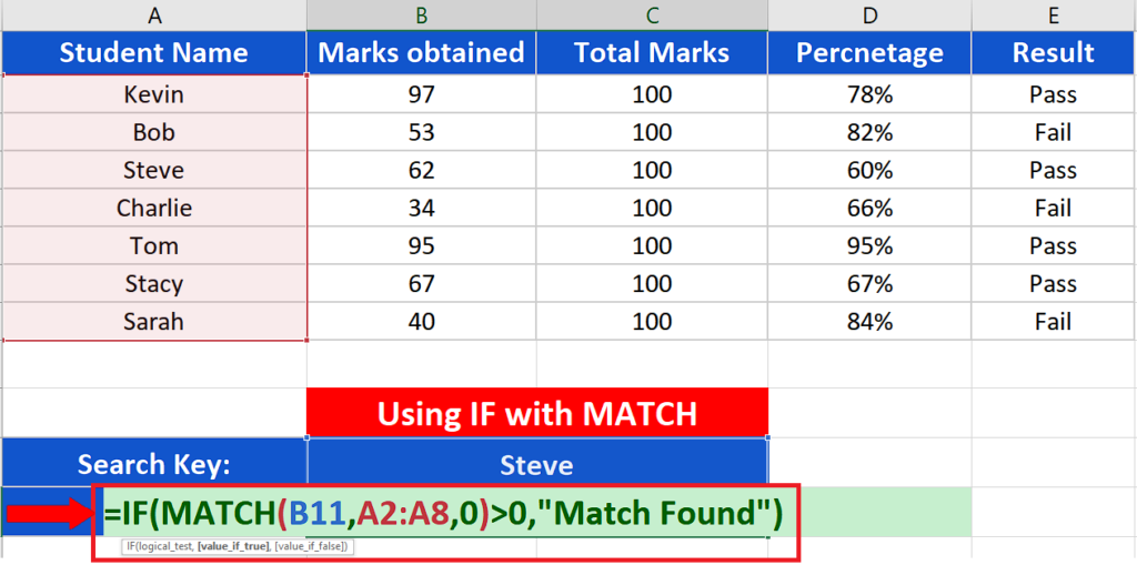
The formula below checks if the value "Apple" is present in the range A1:A10. If it is, the formula returns "True", otherwise, it returns "False".
=IF(ISNUMBER(MATCH("Apple",A1:A10,0)), "True", "False")
How it works:
- The MATCH function looks for the value "Apple" in the range A1:A10.
- The ISNUMBER function checks if the result of the MATCH function is a number. If it is, it means the value was found.
- The IF function checks the result of the ISNUMBER function. If it's true, it returns "True", otherwise, it returns "False".
Method 2: Using MATCH with ISNUMBER Function
Another way to use the MATCH function to determine true or false values is by combining it with the ISNUMBER function. The ISNUMBER function checks if a value is a number and returns true or false accordingly.
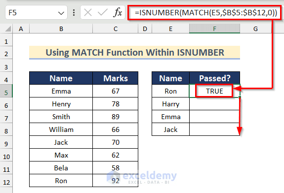
The formula below checks if the value "Apple" is present in the range A1:A10. If it is, the formula returns "True", otherwise, it returns "False".
=ISNUMBER(MATCH("Apple",A1:A10,0))
How it works:
- The MATCH function looks for the value "Apple" in the range A1:A10.
- The ISNUMBER function checks if the result of the MATCH function is a number. If it is, it means the value was found and returns true.
- If the value is not found, the MATCH function returns a #N/A error, which is not a number, so the ISNUMBER function returns false.
Method 3: Using MATCH with INDEX Function
You can also use the MATCH function in combination with the INDEX function to determine true or false values. The INDEX function returns a value from a range based on a row and column number.
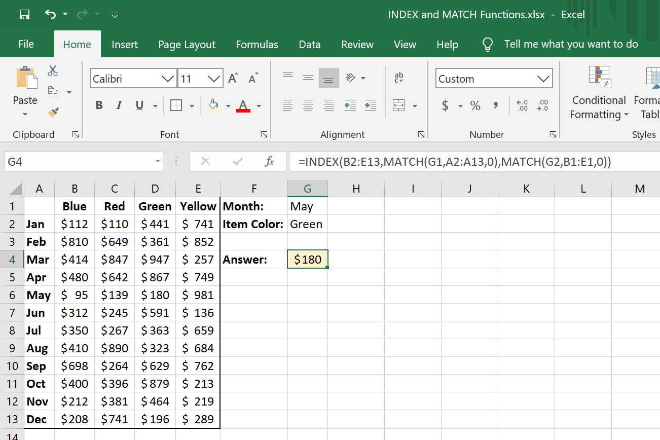
The formula below checks if the value "Apple" is present in the range A1:A10. If it is, the formula returns the value "True", otherwise, it returns the value "False".
=INDEX({"True","False"},ISNUMBER(MATCH("Apple",A1:A10,0))+1)
How it works:
- The MATCH function looks for the value "Apple" in the range A1:A10.
- The ISNUMBER function checks if the result of the MATCH function is a number. If it is, it means the value was found.
- The INDEX function returns the value "True" if the result of the ISNUMBER function is true, otherwise, it returns the value "False".
Method 4: Using MATCH with COUNTIF Function
Another way to use the MATCH function to determine true or false values is by combining it with the COUNTIF function. The COUNTIF function counts the number of cells that meet a certain condition.
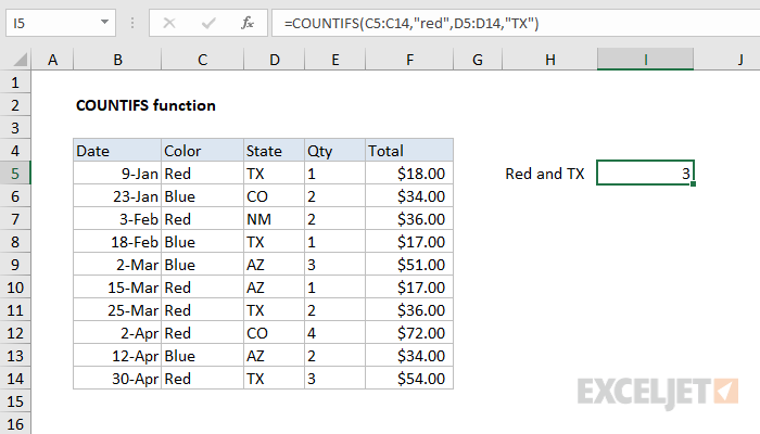
The formula below checks if the value "Apple" is present in the range A1:A10. If it is, the formula returns "True", otherwise, it returns "False".
=IF(COUNTIF(A1:A10,"Apple")>0, "True", "False")
How it works:
- The COUNTIF function counts the number of cells in the range A1:A10 that contain the value "Apple".
- The IF function checks if the result of the COUNTIF function is greater than 0. If it is, it means the value was found, so the formula returns "True".
- If the value is not found, the COUNTIF function returns 0, so the IF function returns "False".
Method 5: Using MATCH with FILTER Function
Finally, you can use the MATCH function in combination with the FILTER function to determine true or false values. The FILTER function filters a range based on a condition.
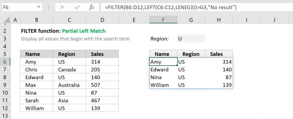
The formula below checks if the value "Apple" is present in the range A1:A10. If it is, the formula returns the value "True", otherwise, it returns the value "False".
=IF(FILTER(A1:A10,A1:A10="Apple")<>"", "True", "False")
How it works:
- The FILTER function filters the range A1:A10 based on the condition that the cells contain the value "Apple".
- The IF function checks if the result of the FILTER function is not blank. If it's not blank, it means the value was found, so the formula returns "True".
- If the value is not found, the FILTER function returns a blank array, so the IF function returns "False".
Gallery of Excel MATCH Function
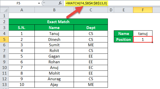
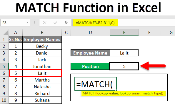
We hope this article has helped you understand how to use the MATCH function in Excel to determine true or false values. With these five methods, you can create powerful formulas that help you analyze and manipulate data in your worksheets. If you have any questions or need further assistance, please don't hesitate to ask.
What is the MATCH function in Excel?
+The MATCH function is a lookup function that returns the position of a value within a range or array.
How do I use the MATCH function with the IF function?
+You can use the MATCH function with the IF function to check if a value is present in a range and return a value accordingly. For example: =IF(ISNUMBER(MATCH("Apple",A1:A10,0)), "True", "False")
What is the difference between the MATCH function and the INDEX function?
+The MATCH function returns the position of a value within a range or array, while the INDEX function returns a value from a range based on a row and column number.
