5 Ways To Use Google Sheets Left Function

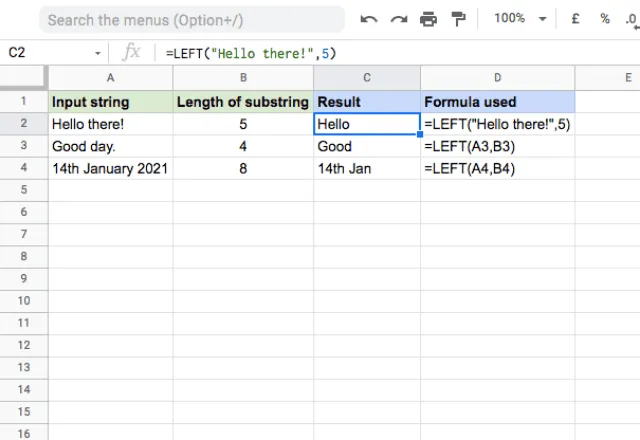
The versatility of Google Sheets! It's an indispensable tool for data analysis, and the LEFT function is one of its most useful features. In this article, we'll explore five ways to use the LEFT function in Google Sheets to extract, manipulate, and analyze data.

Google Sheets has become an essential tool for individuals and businesses alike, offering a wide range of functions to simplify data management. The LEFT function, in particular, is a powerful feature that allows users to extract a specified number of characters from the left side of a text string. This function can be used in various ways to achieve different goals, from data cleaning to data analysis.

In this article, we'll delve into the world of Google Sheets and explore five practical ways to use the LEFT function. Whether you're a beginner or an advanced user, you'll learn how to harness the power of this function to streamline your workflow and gain valuable insights from your data.

What is the LEFT Function in Google Sheets?

Before we dive into the five ways to use the LEFT function, let's briefly explain what it does. The LEFT function in Google Sheets returns a specified number of characters from the left side of a text string. The syntax for the LEFT function is:

LEFT(text, [num_chars])

• text is the text string from which you want to extract characters.
• [num_chars] is the number of characters you want to extract from the left side of the text string. If omitted, the function defaults to 1.

1. Extracting a Specific Number of Characters

One of the most basic uses of the LEFT function is to extract a specific number of characters from a text string. For example, suppose you have a list of product codes in a column, and you want to extract the first three characters of each code. You can use the LEFT function to achieve this.

Assuming your product codes are in column A, you can use the following formula:

=LEFT(A2, 3)

This formula extracts the first three characters from the product code in cell A2. You can then copy this formula down to other cells in the column to extract the first three characters of each product code.

2. Extracting a Fixed-Length Substring

Another way to use the LEFT function is to extract a fixed-length substring from a text string. For instance, suppose you have a list of names in a column, and you want to extract the first five characters of each name. You can use the LEFT function to achieve this.

Assuming your names are in column A, you can use the following formula:

=LEFT(A2, 5)

This formula extracts the first five characters from the name in cell A2. You can then copy this formula down to other cells in the column to extract the first five characters of each name.

3. Extracting a Variable-Length Substring

In some cases, you may need to extract a variable-length substring from a text string. For example, suppose you have a list of email addresses in a column, and you want to extract the domain name (everything after the "@" symbol). You can use the LEFT function in combination with the FIND function to achieve this.

Assuming your email addresses are in column A, you can use the following formula:

=LEFT(A2, FIND("@", A2) - 1)

This formula finds the position of the "@" symbol in the email address in cell A2 and extracts all characters to the left of that position.

4. Removing Unwanted Characters

The LEFT function can also be used to remove unwanted characters from a text string. For example, suppose you have a list of phone numbers in a column, and you want to remove the area code (the first three characters). You can use the LEFT function to achieve this.

Assuming your phone numbers are in column A, you can use the following formula:

=RIGHT(A2, LEN(A2) - 3)

This formula removes the first three characters from the phone number in cell A2. However, if you want to use the LEFT function, you can use the following formula:

=LEFT(A2, LEN(A2) - 3)

This formula extracts all characters except the last three from the phone number in cell A2.

5. Extracting Data from a Specific Position

Finally, the LEFT function can be used to extract data from a specific position in a text string. For example, suppose you have a list of dates in a column, and you want to extract the year (the last four characters). You can use the LEFT function in combination with the LEN function to achieve this.

Assuming your dates are in column A, you can use the following formula:

=RIGHT(A2, 4)

This formula extracts the last four characters from the date in cell A2. However, if you want to use the LEFT function, you can use the following formula:

=LEFT(A2, LEN(A2) - 4)

This formula extracts all characters except the last four from the date in cell A2.

Gallery of Google Sheets LEFT Function Examples

Frequently Asked Questions

In conclusion, the LEFT function in Google Sheets is a powerful feature that can be used in various ways to extract, manipulate, and analyze data. By mastering the LEFT function, you can streamline your workflow, gain valuable insights from your data, and make informed decisions.