5 Ways To Calculate Average In Google Sheets

Calculating averages in Google Sheets is a fundamental task that can help you understand and analyze data more effectively. Whether you're working with a small dataset or a large one, knowing how to calculate averages can provide insights into trends, patterns, and outliers. In this article, we'll explore five ways to calculate averages in Google Sheets, each with its own unique application and benefit.

Google Sheets, as a powerful spreadsheet tool, offers multiple functions and methods to compute averages, catering to different data structures and analysis needs. From the simplest AVERAGE function to more complex formulas that handle errors or specific data conditions, we'll delve into the details of each method.

Method 1: Using the AVERAGE Function

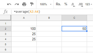
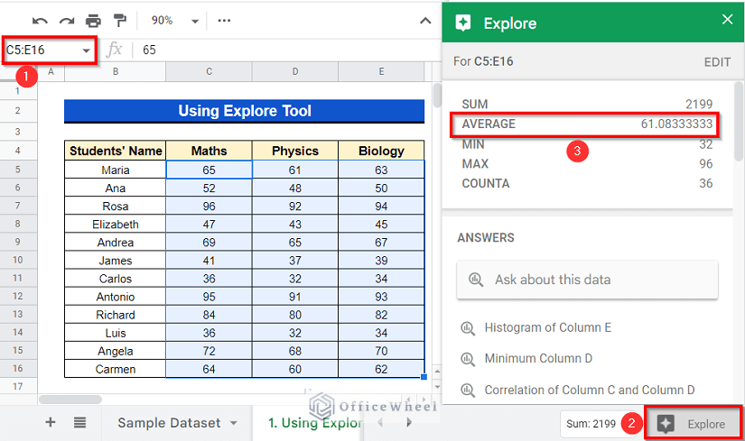
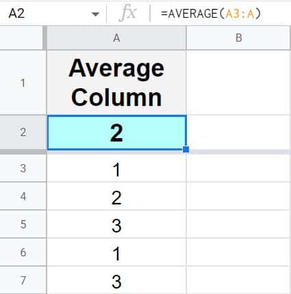
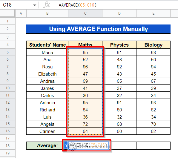
The most straightforward way to calculate an average in Google Sheets is by using the AVERAGE function. This function is easy to use and works well for most averaging tasks. The syntax for the AVERAGE function is:

=AVERAGE(range)

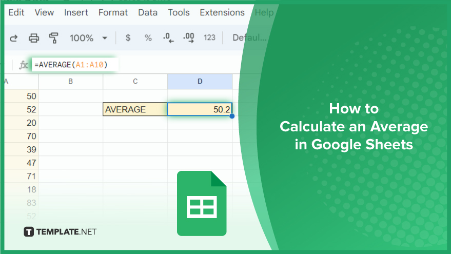
Where "range" is the range of cells you want to average. For example, if you want to average the numbers in cells A1 through A10, your formula would look like this:

=AVERAGE(A1:A10)

This method is quick, straightforward, and ideal for simple averaging tasks. However, it does not ignore errors or empty cells, which might affect your average if present in the range.

Method 2: Calculating Average with Multiple Ranges

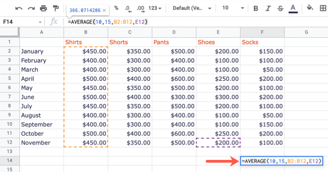
Sometimes, you might need to calculate the average of values spread across multiple ranges. Google Sheets allows you to specify multiple ranges in the AVERAGE function, separated by commas. For example:

=AVERAGE(A1:A5, C1:C5, E1:E5)

This formula averages the values in cells A1 through A5, C1 through C5, and E1 through E5. This method is useful when your data is not contiguous or when you need to average values from different columns or rows.

Method 3: Ignoring Errors with the AVERAGEIF Function

The AVERAGEIF function is another powerful tool in Google Sheets that allows you to calculate averages based on specific conditions. The syntax for the AVERAGEIF function is:

=AVERAGEIF(range, criteria, [average_range])

Where "range" is the range of cells you want to check against the "criteria," and "[average_range]" is the range of cells you want to average. The criteria can be a number, text, or a logical expression.

For example, if you want to average the values in column B where the corresponding values in column A are greater than 10, your formula would look like this:

=AVERAGEIF(A1:A10, ">10", B1:B10)

This method is particularly useful for conditional averaging, where you need to average values based on specific criteria.

Method 4: Using the AVERAGEA Function

The AVERAGEA function in Google Sheets works similarly to the AVERAGE function but with a key difference: it treats text and logical values as 0, whereas the AVERAGE function ignores them. The syntax for the AVERAGEA function is:

=AVERAGEA(range)

Where "range" is the range of cells you want to average.

This method is useful when you have a mix of numeric and non-numeric values in your range and want to include the non-numeric values in your average calculation, treating them as 0.

Method 5: Calculating Moving Averages

A moving average is a calculation that takes the average of a range of values that moves over time. In Google Sheets, you can calculate a moving average using a combination of the AVERAGE function and the OFFSET function.

For example, if you want to calculate a 3-period moving average for the values in column A, starting from row 4, your formula might look like this:

=AVERAGE(OFFSET(A$1, ROW()-1, 0, 3, 1))

This formula calculates the average of the last three values in column A as you move down the rows.

Each of these methods for calculating averages in Google Sheets has its own strengths and is suited for different situations. Whether you're dealing with simple datasets or complex conditional averaging, Google Sheets provides the flexibility and functionality you need.

Gallery of Average Calculation in Google Sheets

Gallery of 5 Ways To Calculate Average In Google Sheets