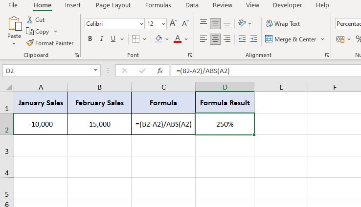
Calculating percentage change in Excel can be a useful skill, especially when you're dealing with financial data, scientific measurements, or any other type of information that requires analyzing changes over time. Percentage change calculations help you understand how much a value has increased or decreased in relation to its original value. In this article, we will explore 5 easy ways to calculate percentage change in Excel.
Calculating percentage change in Excel can be a bit tricky for beginners, but don't worry, we'll break down each method step by step. By the end of this article, you'll be able to confidently calculate percentage changes and analyze your data with ease.

Method 1: Using the Percentage Change Formula
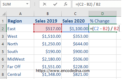
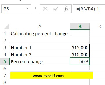
One of the simplest ways to calculate percentage change in Excel is by using the percentage change formula. The formula is as follows:
New Value - Old Value / Old Value
Let's say you have the following data:
| Old Value | New Value |
|---|---|
| 100 | 120 |
To calculate the percentage change, you would use the formula:
=(120-100)/100 =0.2 or 20%
In Excel, you can type this formula into a cell, and it will calculate the percentage change for you. For example, if you have the old value in cell A1 and the new value in cell B1, you would type the following formula into a new cell:
=(B1-A1)/A1
Press Enter, and the formula will calculate the percentage change.
Tips and Variations
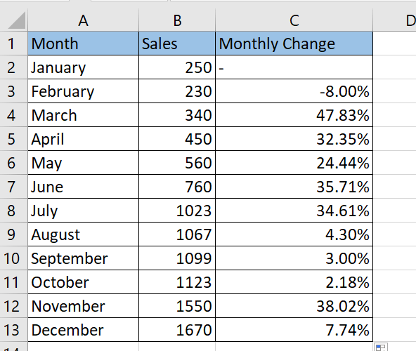
You can format the result as a percentage by selecting the cell and clicking on the "Percent Style" button in the "Number" group of the Home tab.
If you want to calculate the percentage change for multiple cells, you can use an array formula or a formula with an absolute reference.

Method 2: Using the DAX Formula in Power Pivot
If you're using Power Pivot in Excel, you can use the DAX formula to calculate percentage change. The DAX formula is as follows:
% Change = (New Value - Old Value) / Old Value
Let's say you have a table with the following data:
| Date | Sales |
|---|---|
| 2020-01-01 | 100 |
| 2020-01-02 | 120 |
To calculate the percentage change in sales, you would create a new measure in Power Pivot using the following DAX formula:
% Change = VAR OldSales = 'Table'[Sales] VAR NewSales = 'Table'[Sales] RETURN (NewSales - OldSales) / OldSales
You can then add this measure to your pivot table to display the percentage change.
Tips and Variations
You can use the DAX formula to calculate percentage change for multiple columns by modifying the formula to reference the correct columns.
If you want to calculate the percentage change for a specific date range, you can use the DAX formula with a date filter.

Method 3: Using the Excel Percent Change Function
Excel has a built-in function called the Percent Change function that can calculate the percentage change between two values. The function is as follows:
=PERCENTAGECHANGE(old_value, new_value)
Let's say you have the following data:
| Old Value | New Value |
|---|---|
| 100 | 120 |
To calculate the percentage change, you would type the following formula into a cell:
=PERCENTAGECHANGE(A1, B1)
Press Enter, and the formula will calculate the percentage change.
Tips and Variations
You can format the result as a percentage by selecting the cell and clicking on the "Percent Style" button in the "Number" group of the Home tab.
If you want to calculate the percentage change for multiple cells, you can use an array formula or a formula with an absolute reference.

Method 4: Using a Formula with Absolute References
If you want to calculate the percentage change for multiple cells, you can use a formula with absolute references. The formula is as follows:
=((B1-A1)/A1)
Let's say you have the following data:
| Old Value | New Value |
|---|---|
| 100 | 120 |
| 200 | 240 |
To calculate the percentage change, you would type the following formula into a cell:
=((B1-A1)/A1)
Press Enter, and the formula will calculate the percentage change for the first row.
Tips and Variations
You can copy the formula down to the other rows by selecting the cell and pressing Ctrl+C, then selecting the other rows and pressing Ctrl+V.
If you want to calculate the percentage change for multiple columns, you can modify the formula to reference the correct columns.

Method 5: Using a Formula with an Array Formula
If you want to calculate the percentage change for multiple cells, you can use an array formula. The formula is as follows:
=((B1:B10-A1:A10)/A1:A10)
Let's say you have the following data:
| Old Value | New Value |
|---|---|
| 100 | 120 |
| 200 | 240 |
| 300 | 360 |
To calculate the percentage change, you would type the following formula into a cell:
=((B1:B10-A1:A10)/A1:A10)
Press Ctrl+Shift+Enter, and the formula will calculate the percentage change for all the rows.
Tips and Variations
You can format the result as a percentage by selecting the cell and clicking on the "Percent Style" button in the "Number" group of the Home tab.
If you want to calculate the percentage change for multiple columns, you can modify the formula to reference the correct columns.


Conclusion:
Calculating percentage change in Excel is a useful skill that can help you analyze changes over time. In this article, we explored 5 easy ways to calculate percentage change in Excel, including using the percentage change formula, the DAX formula in Power Pivot, the Excel Percent Change function, a formula with absolute references, and an array formula. By following these methods, you can confidently calculate percentage changes and analyze your data with ease.
What is the formula for calculating percentage change?
+The formula for calculating percentage change is (New Value - Old Value) / Old Value.
How do I format the result as a percentage in Excel?
+To format the result as a percentage in Excel, select the cell and click on the "Percent Style" button in the "Number" group of the Home tab.
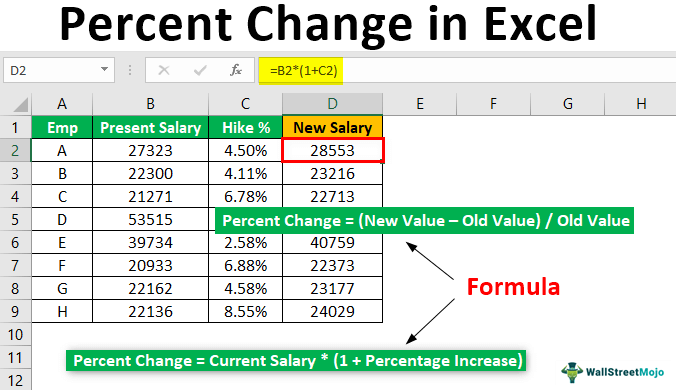


![How to Calculate Percent Change in Excel [Formula]](https://allthings.how/wp-content/uploads/2021/07/allthings.how-how-to-calculate-percent-change-in-excel-formula-image-10.png)

