
The p-value formula in Excel is a statistical tool used to determine the significance of a hypothesis test. It's a crucial concept in data analysis, and Excel provides an efficient way to calculate it. In this article, we'll delve into the world of p-values, exploring what they are, why they're essential, and how to calculate them using Excel.
What is a P-Value?
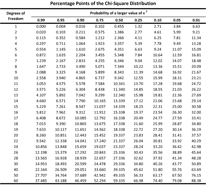
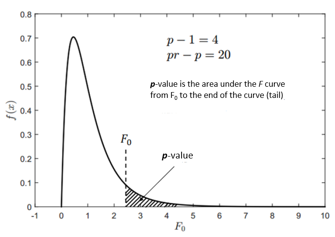
In statistical hypothesis testing, a p-value is a probability value that helps you determine whether the results of your test are due to chance or if they indicate a statistically significant relationship between variables. The p-value is a number between 0 and 1 that represents the probability of observing the results you obtained, assuming that the null hypothesis is true.

The lower the p-value, the stronger the evidence against the null hypothesis. Typically, a p-value of 0.05 or less is considered statistically significant, indicating that the results are unlikely to occur by chance.
Why is the P-Value Important?
The p-value is a crucial concept in statistical analysis because it helps researchers and data analysts determine whether their findings are statistically significant or not. By calculating the p-value, you can:
- Evaluate the strength of evidence: A low p-value indicates strong evidence against the null hypothesis, while a high p-value suggests weak evidence.
- Make informed decisions: P-values help you decide whether to reject the null hypothesis and conclude that there's a statistically significant relationship between variables.
- Avoid Type I errors: By setting a significance level (e.g., 0.05), you can minimize the risk of rejecting a true null hypothesis.
How to Calculate P-Value in Excel
Excel provides several functions to calculate p-values, depending on the type of test you're performing. Here are a few common scenarios:
T-Test P-Value
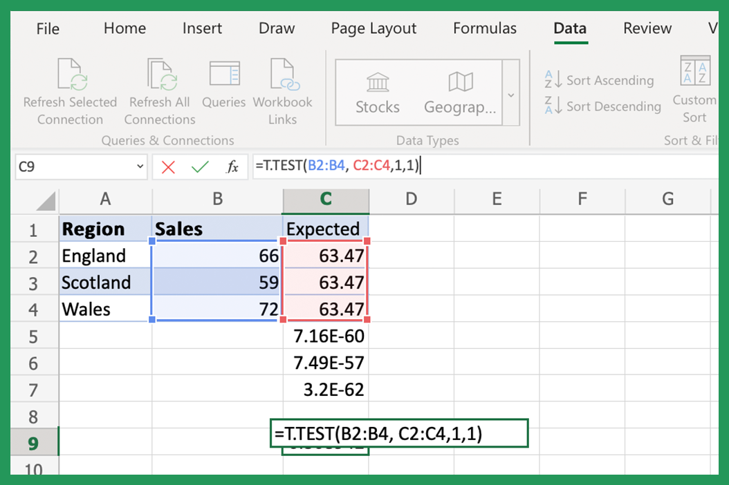
To calculate the p-value for a t-test, you can use the T.TEST function:
- Select the cell where you want to display the p-value.
- Type
=T.TEST(array1, array2, tails, type)and press Enter. - Replace
array1andarray2with the ranges of cells containing your data. - Set
tailsto 1 for a one-tailed test or 2 for a two-tailed test. - Set
typeto 1 for a paired test or 2 for an unpaired test.
Example: =T.TEST(A1:A10, B1:B10, 2, 2)
Chi-Square P-Value
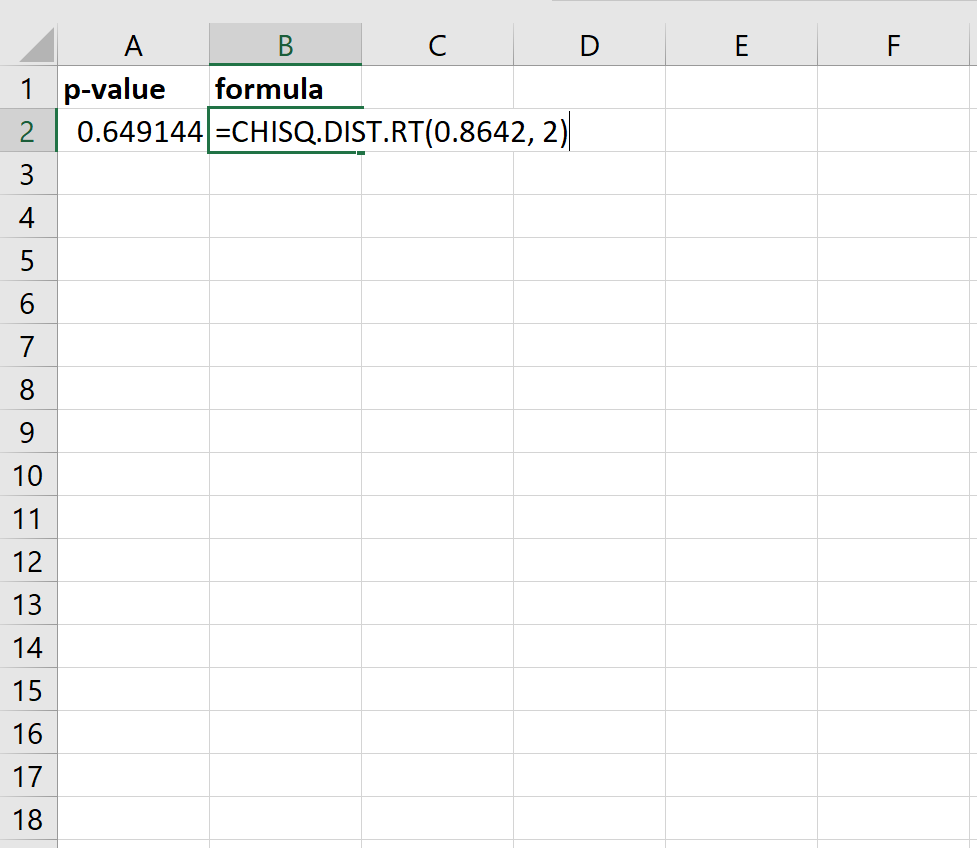
To calculate the p-value for a chi-square test, you can use the CHISQ.TEST function:
- Select the cell where you want to display the p-value.
- Type
=CHISQ.TEST(actual_range, expected_range)and press Enter. - Replace
actual_rangeandexpected_rangewith the ranges of cells containing your data.
Example: =CHISQ.TEST(A1:A10, B1:B10)
Gallery of P-Value Formulas


Frequently Asked Questions
What is the purpose of a p-value?
+The p-value is a probability value that helps you determine whether the results of your test are due to chance or if they indicate a statistically significant relationship between variables.
What is the significance level?
+The significance level, typically set at 0.05, is the maximum probability of rejecting a true null hypothesis.
How do I interpret a p-value?
+A low p-value (e.g., 0.05 or less) indicates strong evidence against the null hypothesis, while a high p-value (e.g., greater than 0.05) suggests weak evidence.
In conclusion, the p-value formula in Excel is a powerful tool for statistical analysis. By understanding how to calculate and interpret p-values, you can make informed decisions and draw meaningful conclusions from your data. Remember to choose the correct formula based on your test type and to set a significance level to avoid Type I errors. Happy calculating!