The world of Google Sheets formulas can be overwhelming, especially for those new to the platform. Among the many formulas available, the Index Match formula stands out as a powerful and versatile tool for data analysis and manipulation. In this article, we'll delve into the world of Index Match, exploring its benefits, how it works, and providing practical examples to help you master this essential formula.
Mastering Index Match can revolutionize the way you work with data in Google Sheets. This formula allows you to look up and retrieve data from a table based on specific criteria, making it a valuable asset for data analysis, reporting, and more. By the end of this article, you'll be equipped with the knowledge to harness the full potential of Index Match and take your Google Sheets skills to the next level.
Understanding the Index Match Formula
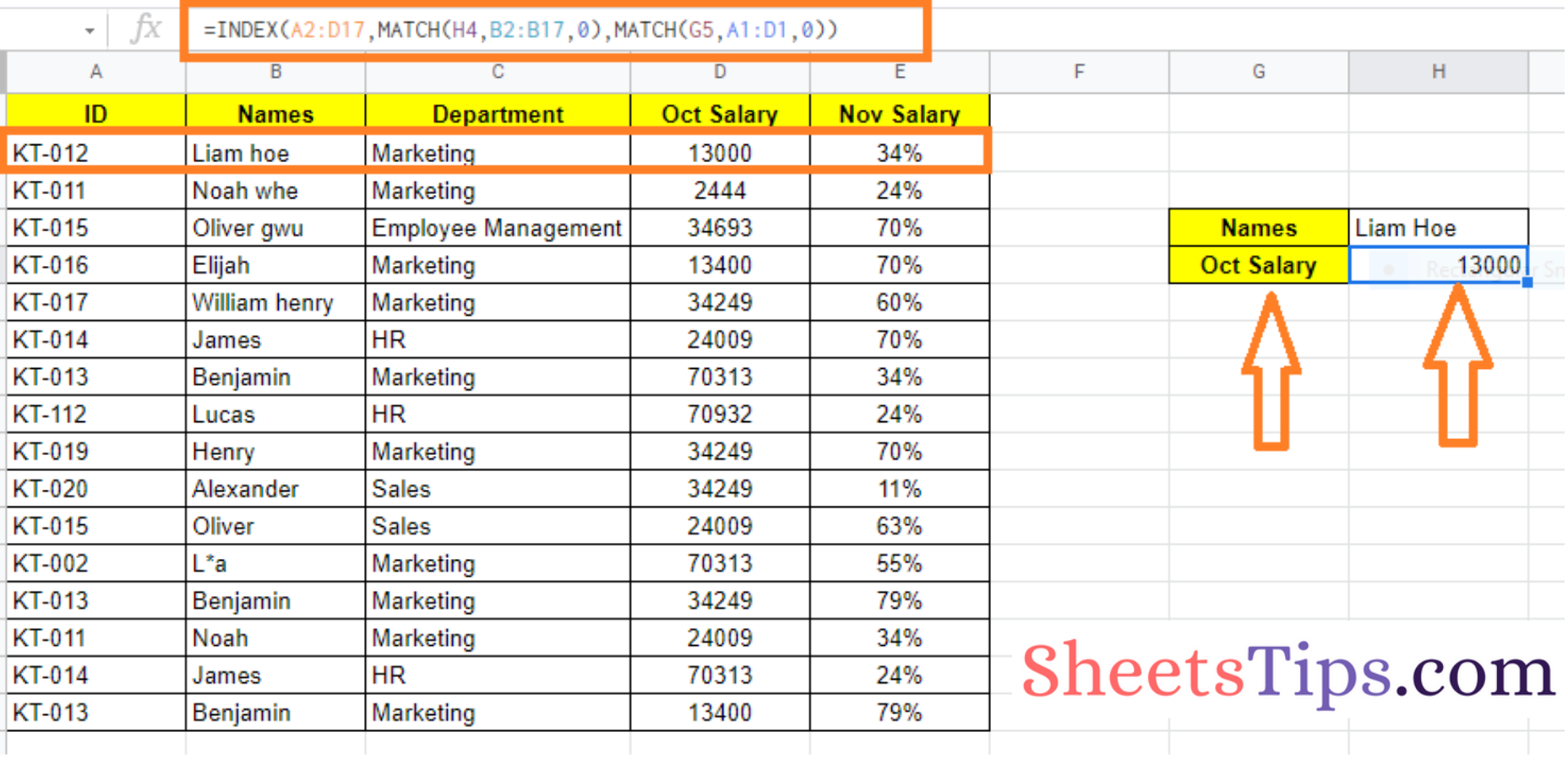
The Index Match formula is a combination of two separate formulas: Index and Match. To understand how it works, let's break down each component:
- Index: The Index formula returns a value from a specified range or array based on a row and column number.
- Match: The Match formula returns the relative position of a value within a range or array.
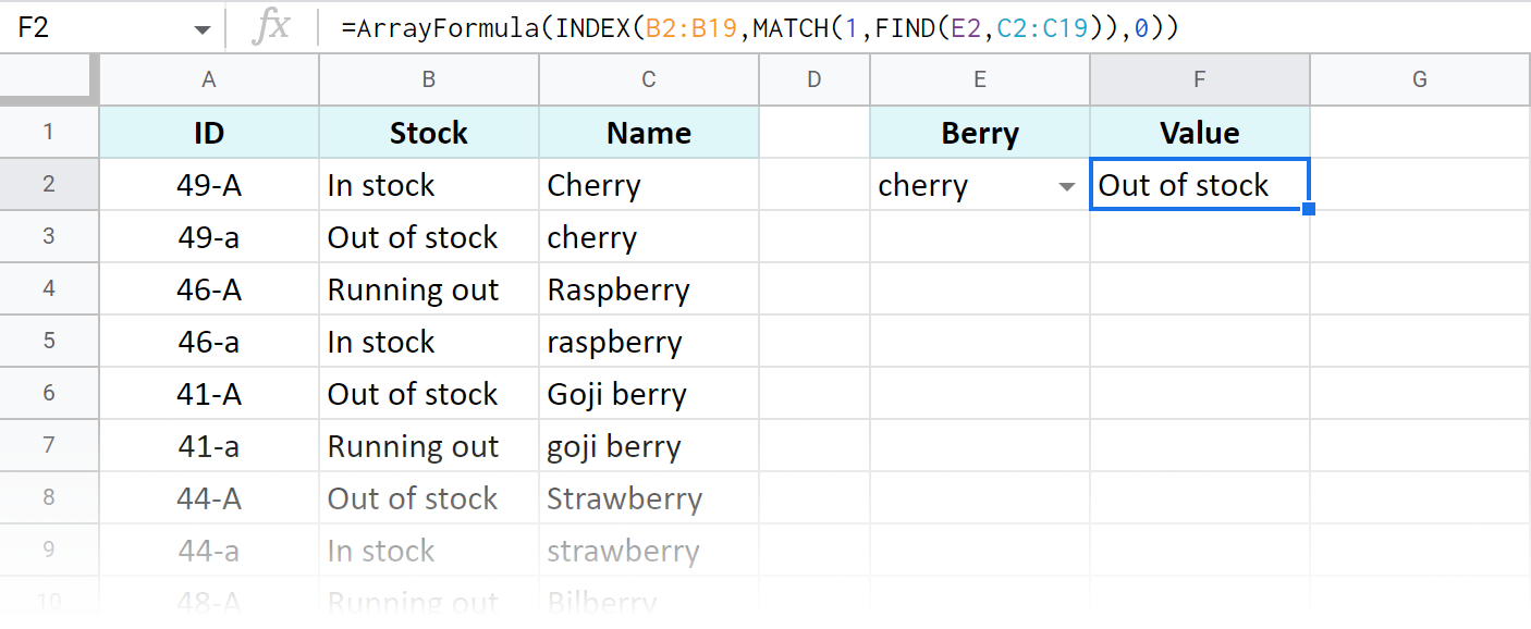
When combined, the Index Match formula uses the Match formula to find the relative position of a value within a range and then uses the Index formula to return the corresponding value from another range.
Basic Syntax of Index Match Formula
The basic syntax of the Index Match formula is as follows:
=INDEX(range1, MATCH(value, range2, [match_type])
range1: The range of cells that contains the value you want to return.value: The value you want to look up.range2: The range of cells that contains the value you want to look up.[match_type]: Optional parameter that specifies the type of match (exact, approximate, or wildcard).

Practical Examples of Index Match Formula
To illustrate the power of the Index Match formula, let's explore some practical examples:
Example 1: Simple Lookup
Suppose you have a table with employee names and their corresponding department numbers. You want to find the department number for a specific employee.
| Employee Name | Department Number |
|---|---|
| John Smith | 101 |
| Jane Doe | 102 |
| Bob Johnson | 103 |
Using the Index Match formula, you can look up the department number for John Smith as follows:
=INDEX(B:B, MATCH("John Smith", A:A, 0))
B:B: The range of cells that contains the department numbers."John Smith": The value you want to look up.A:A: The range of cells that contains the employee names.0: Exact match.
The formula returns the department number for John Smith, which is 101.
Example 2: Multiple Criteria Lookup
Suppose you have a table with sales data, including region, product, and sales amount. You want to find the sales amount for a specific region and product.
| Region | Product | Sales Amount |
|---|---|---|
| North | Product A | 1000 |
| North | Product B | 2000 |
| South | Product A | 3000 |
| South | Product B | 4000 |
Using the Index Match formula, you can look up the sales amount for the North region and Product A as follows:
=INDEX(C:C, MATCH(1, (A:A="North") \* (B:B="Product A"), 0))
C:C: The range of cells that contains the sales amounts.1: The value you want to look up (1 represents the intersection of the two criteria).(A:A="North") \* (B:B="Product A"): The criteria for the lookup (region and product).0: Exact match.
The formula returns the sales amount for the North region and Product A, which is 1000.
Benefits of Using Index Match Formula
The Index Match formula offers several benefits over other lookup formulas, including:
- Flexibility: Can be used for simple and complex lookups.
- Power: Can handle multiple criteria and ranges.
- Speed: Faster than other lookup formulas, especially for large datasets.

Common Errors and Troubleshooting
When working with the Index Match formula, you may encounter errors or issues. Here are some common errors and troubleshooting tips:
- #N/A Error: This error occurs when the formula cannot find a match. Check the data and ensure that the value you're looking up exists in the range.
- #VALUE! Error: This error occurs when the formula encounters an invalid value. Check the data and ensure that it's in the correct format.
Best Practices for Using Index Match Formula
To get the most out of the Index Match formula, follow these best practices:
- Use absolute references: Use absolute references for the ranges to ensure that the formula works correctly even when the data changes.
- Use named ranges: Use named ranges to make the formula more readable and easier to maintain.
- Test the formula: Test the formula thoroughly to ensure that it's working correctly and returning the expected results.

Conclusion
The Index Match formula is a powerful tool for data analysis and manipulation in Google Sheets. By mastering this formula, you can unlock the full potential of your data and take your Google Sheets skills to the next level. Remember to use absolute references, named ranges, and test the formula thoroughly to ensure that it's working correctly. With practice and patience, you'll become proficient in using the Index Match formula and be able to tackle even the most complex data challenges.

What's Next?
Now that you've mastered the Index Match formula, it's time to take your Google Sheets skills to the next level. Here are some next steps:
- Explore other lookup formulas: Learn about other lookup formulas, such as VLOOKUP and HLOOKUP, and when to use them.
- Practice with real-world examples: Practice using the Index Match formula with real-world examples to reinforce your understanding.
- Learn advanced Google Sheets techniques: Learn advanced Google Sheets techniques, such as using arrays and scripting, to take your skills to the next level.
By following these next steps, you'll become a Google Sheets expert and be able to tackle even the most complex data challenges.


What is the Index Match formula in Google Sheets?
+The Index Match formula is a combination of two separate formulas: Index and Match. It uses the Match formula to find the relative position of a value within a range and then uses the Index formula to return the corresponding value from another range.
How do I use the Index Match formula in Google Sheets?
+To use the Index Match formula in Google Sheets, follow these steps: 1. Select the cell where you want to display the result. 2. Type "=INDEX(" and select the range of cells that contains the value you want to return. 3. Type ", MATCH(" and select the value you want to look up. 4. Type ", " and select the range of cells that contains the value you want to look up. 5. Type ", [match_type])" and specify the type of match (exact, approximate, or wildcard). 6. Press Enter to display the result.
What are the benefits of using the Index Match formula in Google Sheets?
+The Index Match formula offers several benefits, including flexibility, power, and speed. It can be used for simple and complex lookups, handles multiple criteria and ranges, and is faster than other lookup formulas, especially for large datasets.