5 Ways To Use Conditional Formatting With Dates In Excel

When working with dates in Excel, it's often necessary to highlight specific dates or date ranges to make your data more understandable and easier to analyze. One of the most effective ways to achieve this is by using conditional formatting with dates in Excel. In this article, we'll explore five ways to use conditional formatting with dates in Excel, including how to highlight dates within a specific range, how to identify upcoming dates, and more.

Conditional formatting is a powerful feature in Excel that allows you to format cells based on specific conditions, such as the value in a cell or the formula that you specify. When working with dates, you can use conditional formatting to highlight cells that meet certain criteria, such as dates within a specific range or dates that are within a certain number of days from the current date.

Highlighting Dates within a Specific Range

One common use of conditional formatting with dates is to highlight cells that contain dates within a specific range. For example, you might want to highlight all dates that occur within the next 30 days.

To achieve this, follow these steps:

1. Select the cells that contain the dates you want to format.
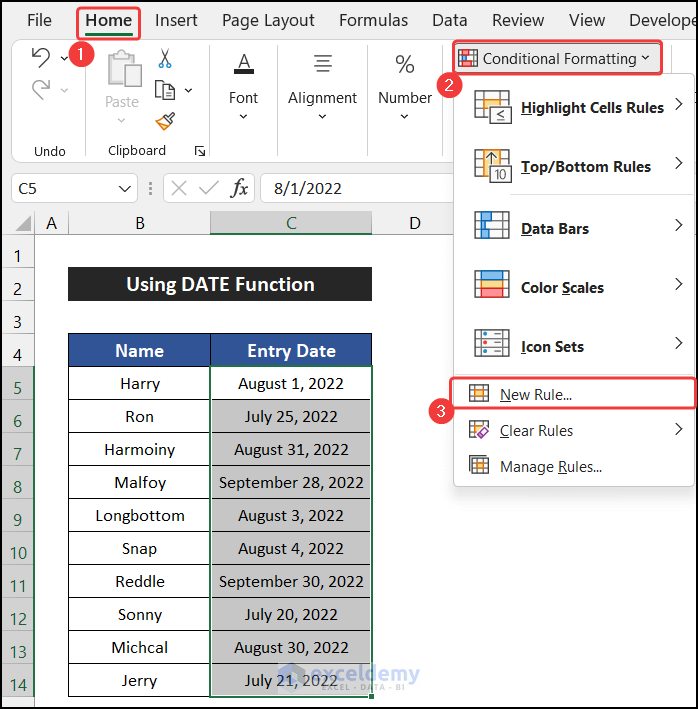
2. Go to the Home tab in the Excel ribbon.
3. Click on the Conditional Formatting button in the Styles group.
4. Select "New Rule" from the drop-down menu.
5. Choose "Use a formula to determine which cells to format."
6. Enter the following formula: =AND(A1>=TODAY(), A1<=TODAY()+30)
7. Click on the Format button and select the desired format.
8. Click OK to apply the rule.

This formula will highlight all cells that contain dates within the next 30 days from the current date.

Highlighting Upcoming Dates

Another common use of conditional formatting with dates is to highlight cells that contain upcoming dates. For example, you might want to highlight all dates that occur within the next week.

To achieve this, follow these steps:

1. Select the cells that contain the dates you want to format.
2. Go to the Home tab in the Excel ribbon.
3. Click on the Conditional Formatting button in the Styles group.
4. Select "New Rule" from the drop-down menu.
5. Choose "Use a formula to determine which cells to format."
6. Enter the following formula: =A1>=TODAY()
7. Click on the Format button and select the desired format.
8. Click OK to apply the rule.

This formula will highlight all cells that contain dates that are later than the current date.

Highlighting Dates within a Specific Month

You can also use conditional formatting to highlight cells that contain dates within a specific month. For example, you might want to highlight all dates that occur in the current month.

To achieve this, follow these steps:

1. Select the cells that contain the dates you want to format.
2. Go to the Home tab in the Excel ribbon.
3. Click on the Conditional Formatting button in the Styles group.
4. Select "New Rule" from the drop-down menu.
5. Choose "Use a formula to determine which cells to format."
6. Enter the following formula: =MONTH(A1)=MONTH(TODAY())
7. Click on the Format button and select the desired format.
8. Click OK to apply the rule.

This formula will highlight all cells that contain dates within the current month.

Highlighting Dates within a Specific Quarter

You can also use conditional formatting to highlight cells that contain dates within a specific quarter. For example, you might want to highlight all dates that occur within the current quarter.

To achieve this, follow these steps:

1. Select the cells that contain the dates you want to format.
2. Go to the Home tab in the Excel ribbon.
3. Click on the Conditional Formatting button in the Styles group.
4. Select "New Rule" from the drop-down menu.
5. Choose "Use a formula to determine which cells to format."
6. Enter the following formula: =ROUNDUP(MONTH(A1)/3)=ROUNDUP(MONTH(TODAY())/3)
7. Click on the Format button and select the desired format.
8. Click OK to apply the rule.

This formula will highlight all cells that contain dates within the current quarter.

Highlighting Dates within a Specific Year

Finally, you can use conditional formatting to highlight cells that contain dates within a specific year. For example, you might want to highlight all dates that occur within the current year.

To achieve this, follow these steps:

1. Select the cells that contain the dates you want to format.
2. Go to the Home tab in the Excel ribbon.
3. Click on the Conditional Formatting button in the Styles group.
4. Select "New Rule" from the drop-down menu.
5. Choose "Use a formula to determine which cells to format."
6. Enter the following formula: =YEAR(A1)=YEAR(TODAY())
7. Click on the Format button and select the desired format.
8. Click OK to apply the rule.

This formula will highlight all cells that contain dates within the current year.

We hope this article has helped you to learn more about using conditional formatting with dates in Excel. With these techniques, you can make your data more understandable and easier to analyze, and improve your overall productivity and efficiency in Excel.

Gallery of 5 Ways To Use Conditional Formatting With Dates In Excel