3 Ways To Remove Last Character In Google Sheets

The importance of data manipulation in Google Sheets cannot be overstated. One common task that users often face is removing the last character from a cell or a range of cells. Whether it's to clean up data, format it for further analysis, or prepare it for other applications, knowing how to efficiently remove characters is a valuable skill. In this article, we'll delve into three methods to remove the last character in Google Sheets, exploring their applications, limitations, and providing step-by-step instructions.

Understanding the Need to Remove Last Characters

Before diving into the methods, it's essential to understand why removing the last character might be necessary. This task is often required when dealing with imported data that contains trailing characters, such as commas, periods, or other punctuation marks, which can interfere with data analysis or formatting. Removing these characters can make your data cleaner and more manageable.

Method 1: Using the LEFT Function

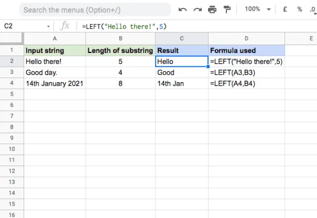
The LEFT function in Google Sheets is primarily used to extract a specified number of characters from the left side of a string. However, you can also use it to remove the last character by extracting all characters except the last one. The syntax for the LEFT function is LEFT(text, [number_of_chars]), where text is the string from which you want to extract characters, and [number_of_chars] is the number of characters you want to extract.

To remove the last character using the LEFT function, you would use the formula:

=LEFT(A1, LEN(A1)-1)

Here, A1 is the cell containing the text from which you want to remove the last character. LEN(A1) calculates the total length of the string, and subtracting 1 gives you the length of the string minus the last character.

How to Apply the LEFT Function:

1. Select the cell where you want to display the result.
2. Type =LEFT(A1, LEN(A1)-1), replacing A1 with the cell containing the text you want to edit.
3. Press Enter to apply the formula.

Method 2: Using the REGEXREPLACE Function

The REGEXREPLACE function in Google Sheets allows you to replace text using regular expressions. While its primary use is for replacing specified patterns, you can also use it to remove the last character from a string by replacing the last character with an empty string.

The syntax for the REGEXREPLACE function is REGEXREPLACE(text, regular_expression, replacement), where text is the string you want to edit, regular_expression is the pattern you want to match (in this case, the last character), and replacement is what you want to replace the matched pattern with (an empty string to effectively remove the character).

To remove the last character using REGEXREPLACE, you would use the formula:

=REGEXREPLACE(A1, ".${content}quot;, "")

Here, A1 is the cell containing the text from which you want to remove the last character. ".${content}quot; is the regular expression that matches the last character of the string (the dot . matches any character, and the dollar sign $ anchors the match to the end of the string), and "" is the empty string that replaces the last character.

How to Apply the REGEXREPLACE Function:

1. Select the cell where you want to display the result.
2. Type =REGEXREPLACE(A1, ".${content}quot;, ""), replacing A1 with the cell containing the text you want to edit.
3. Press Enter to apply the formula.

Method 3: Using the RIGHT and LEN Functions Together

While the RIGHT function is used to extract a specified number of characters from the right side of a string, combining it with the LEN function allows you to remove the last character by extracting all characters except the last one.

The syntax for this method would be:

=RIGHT(A1, LEN(A1)-1)

However, this approach is less intuitive compared to using the LEFT function, as the RIGHT function's nature is to start from the right, not from the left. Therefore, it's generally more straightforward and logical to use the LEFT function for removing the last character.

Gallery of Removing Last Character in Google Sheets

Removing the last character from a string in Google Sheets is a common requirement that can be achieved through various methods. The LEFT function combined with LEN, the REGEXREPLACE function, and even a combination of the RIGHT and LEN functions can all be used to remove the last character. However, the LEFT function method stands out as the most straightforward and logical approach. By mastering these techniques, users can efficiently manage and analyze their data in Google Sheets.

Gallery of 3 Ways To Remove Last Character In Google Sheets