5 Ways To Query Another Sheet In Google Sheets

Google Sheets is a powerful tool for data analysis and manipulation. One of its most useful features is the ability to query data from another sheet within the same spreadsheet or even from a different spreadsheet. This allows you to consolidate data, create reports, and perform complex analysis across multiple sheets. In this article, we will explore five ways to query another sheet in Google Sheets.

Method 1: Using the QUERY Function

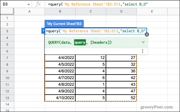
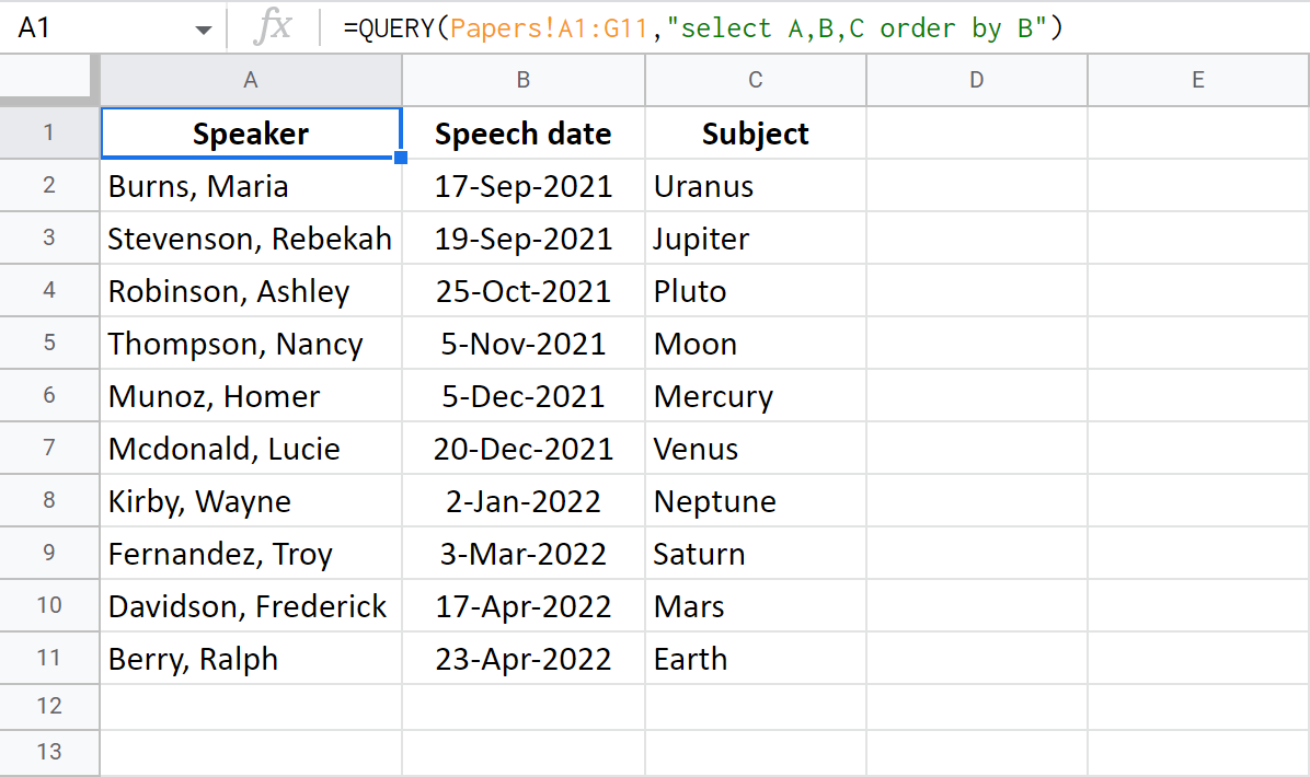
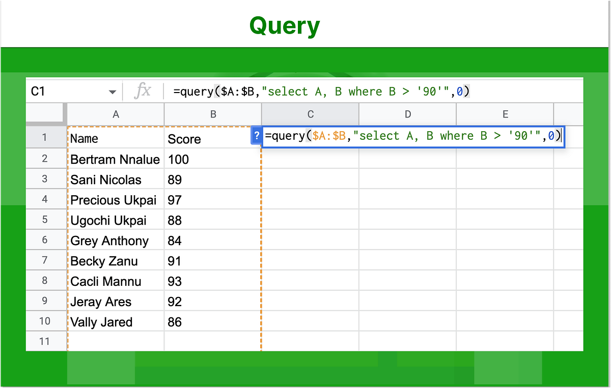
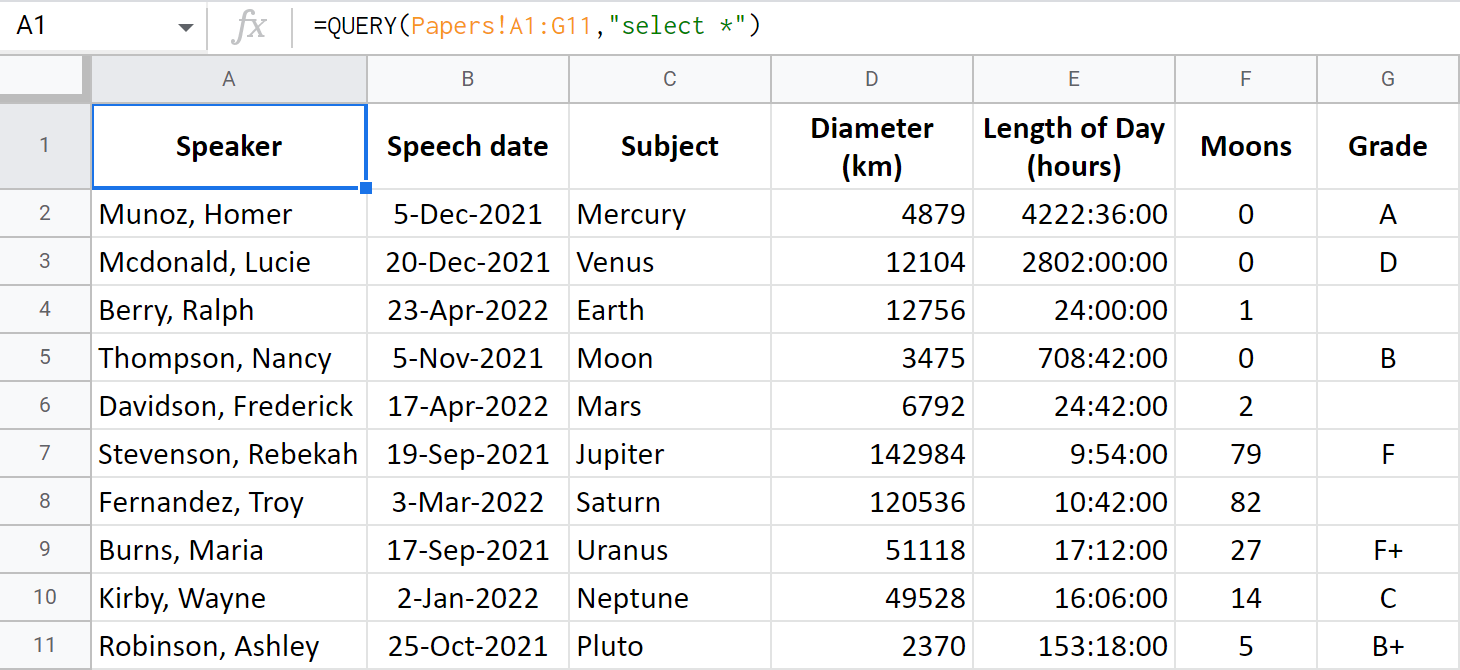
The QUERY function is a powerful tool in Google Sheets that allows you to query data from another sheet or even from a different spreadsheet. The syntax for the QUERY function is as follows:

=QUERY(range, query, [headers])

Where:

range is the range of cells that you want to query.
query is the query that you want to execute.
[headers] is an optional parameter that specifies whether the first row of the range should be treated as headers.

For example, suppose you have a sheet called "Data" with the following data:

Name	Age	Country
John	25	USA
Mary	31	UK
David	42	Australia

You can use the following QUERY function to retrieve all rows where the age is greater than 30:

=QUERY(Data!A:C, "SELECT * WHERE C > 30", 0)

This will return the following result:

Name	Age	Country
Mary	31	UK
David	42	Australia

Method 2: Using the IMPORTRANGE Function

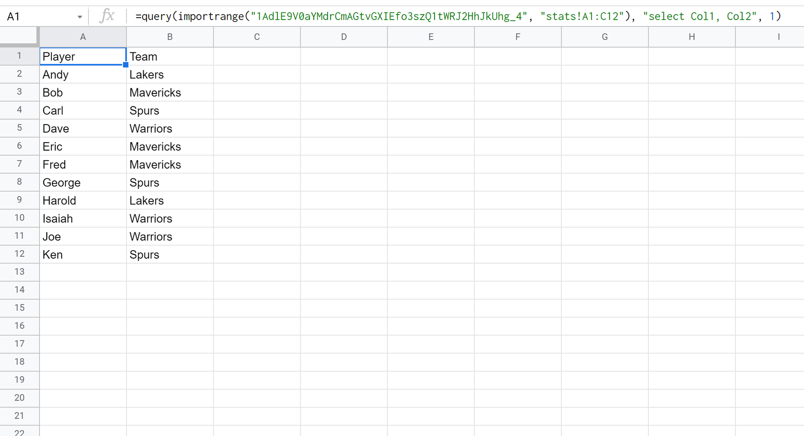
The IMPORTRANGE function allows you to import data from another sheet or even from a different spreadsheet. The syntax for the IMPORTRANGE function is as follows:

=IMPORTRANGE(spreadsheet_url, range_string)

Where:

spreadsheet_url is the URL of the spreadsheet that you want to import data from.
range_string is the range of cells that you want to import.

For example, suppose you have a sheet called "Data" in a different spreadsheet with the following data:

Name	Age	Country
John	25	USA
Mary	31	UK
David	42	Australia

You can use the following IMPORTRANGE function to import all data from the "Data" sheet:

=IMPORTRANGE("https://docs.google.com/spreadsheets/d/your_spreadsheet_id", "Data!A:C")

This will import all data from the "Data" sheet into your current sheet.

Method 3: Using the VLOOKUP Function

The VLOOKUP function allows you to look up data in another sheet or even from a different spreadsheet. The syntax for the VLOOKUP function is as follows:

=VLOOKUP(lookup_value, table_array, col_index_num, [range_lookup])

Where:

lookup_value is the value that you want to look up.
table_array is the range of cells that you want to search.
col_index_num is the column number that you want to return.
[range_lookup] is an optional parameter that specifies whether you want to perform an exact match or an approximate match.

For example, suppose you have a sheet called "Data" with the following data:

Name	Age	Country
John	25	USA
Mary	31	UK
David	42	Australia

You can use the following VLOOKUP function to look up the age of John:

=VLOOKUP("John", Data!A:C, 2, FALSE)

This will return the value "25".

Method 4: Using the INDEX and MATCH Functions

The INDEX and MATCH functions allow you to look up data in another sheet or even from a different spreadsheet. The syntax for the INDEX and MATCH functions is as follows:

=INDEX(range, MATCH(lookup_value, range, [match_type])

Where:

range is the range of cells that you want to search.
lookup_value is the value that you want to look up.
[match_type] is an optional parameter that specifies the type of match that you want to perform.

For example, suppose you have a sheet called "Data" with the following data:

Name	Age	Country
John	25	USA
Mary	31	UK
David	42	Australia

You can use the following INDEX and MATCH functions to look up the age of John:

=INDEX(Data!B:B, MATCH("John", Data!A:A, 0))

This will return the value "25".

Method 5: Using the FILTER Function

The FILTER function allows you to filter data in another sheet or even from a different spreadsheet. The syntax for the FILTER function is as follows:

=FILTER(range, condition)

Where:

range is the range of cells that you want to filter.
condition is the condition that you want to apply to the data.

For example, suppose you have a sheet called "Data" with the following data:

Name	Age	Country
John	25	USA
Mary	31	UK
David	42	Australia

You can use the following FILTER function to filter all rows where the age is greater than 30:

=FILTER(Data!A:C, Data!B:B > 30)

This will return the following result:

Name	Age	Country
Mary	31	UK
David	42	Australia

Gallery of Google Sheets Query Functions

What is the best way to query another sheet in Google Sheets?

The best way to query another sheet in Google Sheets depends on your specific needs and goals. If you want to perform complex queries, the `QUERY` function may be the best option. If you want to import data from another sheet or spreadsheet, the `IMPORTRANGE` function may be the best option.

How do I use the `QUERY` function in Google Sheets?

The `QUERY` function in Google Sheets allows you to query data from another sheet or even from a different spreadsheet. The syntax for the `QUERY` function is as follows: `=QUERY(range, query, [headers])`. Where `range` is the range of cells that you want to query, `query` is the query that you want to execute, and `[headers]` is an optional parameter that specifies whether the first row of the range should be treated as headers.

How do I use the `IMPORTRANGE` function in Google Sheets?

The `IMPORTRANGE` function in Google Sheets allows you to import data from another sheet or even from a different spreadsheet. The syntax for the `IMPORTRANGE` function is as follows: `=IMPORTRANGE(spreadsheet_url, range_string)`. Where `spreadsheet_url` is the URL of the spreadsheet that you want to import data from, and `range_string` is the range of cells that you want to import.