5 Ways To Calculate Average In Google Sheets Ignoring 0

Calculating the average of a dataset is a common task in data analysis, and Google Sheets provides several ways to do this. However, when working with datasets that contain zeros, you may want to exclude these values from the calculation to get a more accurate representation of the average. Here are 5 ways to calculate the average in Google Sheets, ignoring zeros.

Why Ignore Zeros? Before we dive into the methods, it's essential to understand why ignoring zeros might be necessary. Zeros can significantly skew the average, especially if they represent missing or invalid data. By excluding zeros from the calculation, you can get a more accurate representation of the average value in your dataset.

Method 1: Using the AVERAGEIF Function

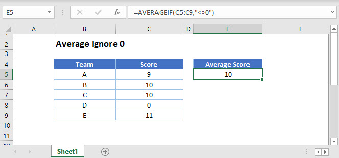
The AVERAGEIF function in Google Sheets allows you to calculate the average of a range of cells, based on a specific condition. To ignore zeros, you can use the following formula:

=AVERAGEIF(range, ">0")

Assuming your data is in the range A1:A10, this formula will calculate the average of all non-zero values in that range.

Method 2: Using the FILTER Function

The FILTER function is a powerful tool in Google Sheets that allows you to filter data based on specific conditions. To calculate the average, ignoring zeros, you can use the following formula:

=AVERAGE(FILTER(range, range>0))

Again, assuming your data is in the range A1:A10, this formula will filter out the zeros and calculate the average of the remaining values.

Method 3: Using the SUM and COUNTIF Functions

This method involves using the SUM and COUNTIF functions in combination to calculate the average, ignoring zeros. The formula is as follows:

=SUM(range) / COUNTIF(range, ">0")

This formula calculates the sum of all values in the range and then divides it by the count of non-zero values in the same range.

Method 4: Using the AVERAGE Function with a Conditional Statement

You can also use the AVERAGE function with a conditional statement to ignore zeros. The formula is as follows:

=AVERAGE(IF(range>0, range, ""))

This formula uses the IF statement to check if each value in the range is greater than zero. If it is, the value is included in the average calculation; otherwise, it is ignored.

Method 5: Using the Query Function

The Query function in Google Sheets is a powerful tool that allows you to perform complex data analysis tasks. To calculate the average, ignoring zeros, you can use the following formula:

=QUERY(range, "SELECT AVG(Col1) WHERE Col1 > 0")

Assuming your data is in the range A1:A10, this formula will calculate the average of all non-zero values in that range.

Conclusion

In this article, we've explored 5 ways to calculate the average in Google Sheets, ignoring zeros. Each method has its own advantages and disadvantages, and the choice of which one to use will depend on your specific use case. By excluding zeros from the calculation, you can get a more accurate representation of the average value in your dataset.

Do you have any questions about calculating averages in Google Sheets? Share them in the comments below!

Gallery of 5 Ways To Calculate Average In Google Sheets Ignoring 0