5 Ways To Dynamically Reference Excel Table Columns

Working with Excel tables can be a daunting task, especially when dealing with large datasets. One of the most efficient ways to manage and analyze data in Excel is by using tables. However, referencing columns in an Excel table can be tedious, especially when the table structure changes. In this article, we will explore five ways to dynamically reference Excel table columns, making your data analysis more efficient and accurate.

Dynamically referencing columns in an Excel table can save you time and reduce errors. Whether you are creating formulas, charts, or pivot tables, being able to reference columns dynamically can make a huge difference in your productivity. In this article, we will cover the following methods:

Using the Tabela notation
Employing the INDEX and MATCH functions
Utilizing the OFFSET function
Leveraging the XLOOKUP function
Creating dynamic named ranges

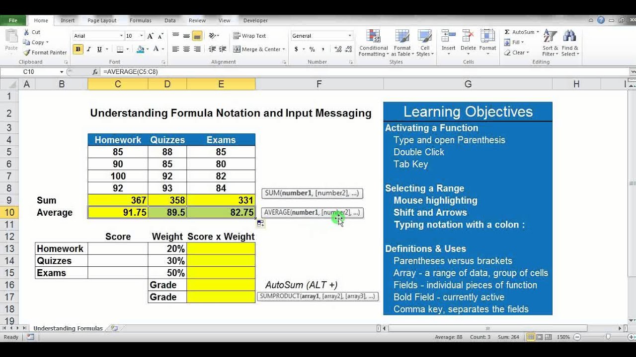
Using the Tabela notation

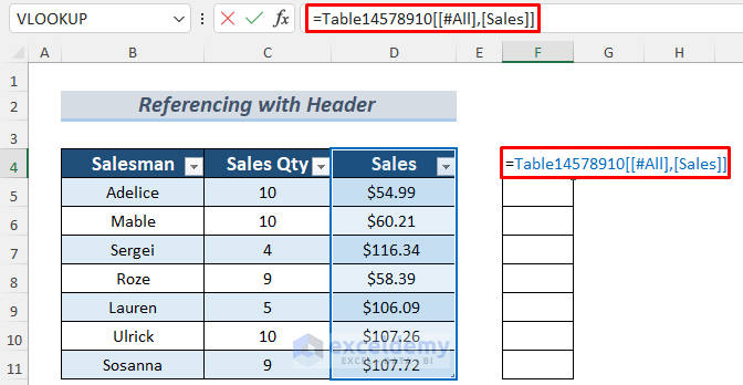
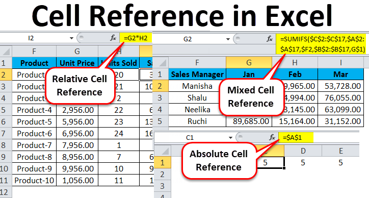
One of the simplest ways to dynamically reference an Excel table column is by using the Tabela notation. This method involves referencing the column using the table name followed by the column name. For example, if you have a table named Sales with a column named Region, you can reference the Region column using the following formula:

=Sales[Region]

This notation is not only easy to read but also dynamic, meaning that if you add or remove columns from the table, the formula will automatically adjust.

Employing the INDEX and MATCH functions

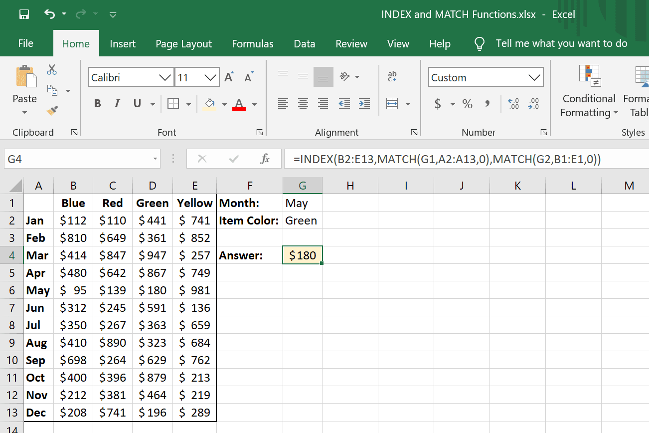
Another way to dynamically reference an Excel table column is by using the INDEX and MATCH functions. The INDEX function returns a value at a specified position in a range, while the MATCH function returns the relative position of a value within a range.

To dynamically reference a column using these functions, you can use the following formula:

=INDEX(Sales, 0, MATCH("Region", Sales[#Headers], 0))

In this formula, the INDEX function returns the entire column, while the MATCH function returns the relative position of the Region column within the table headers.

Utilizing the OFFSET function

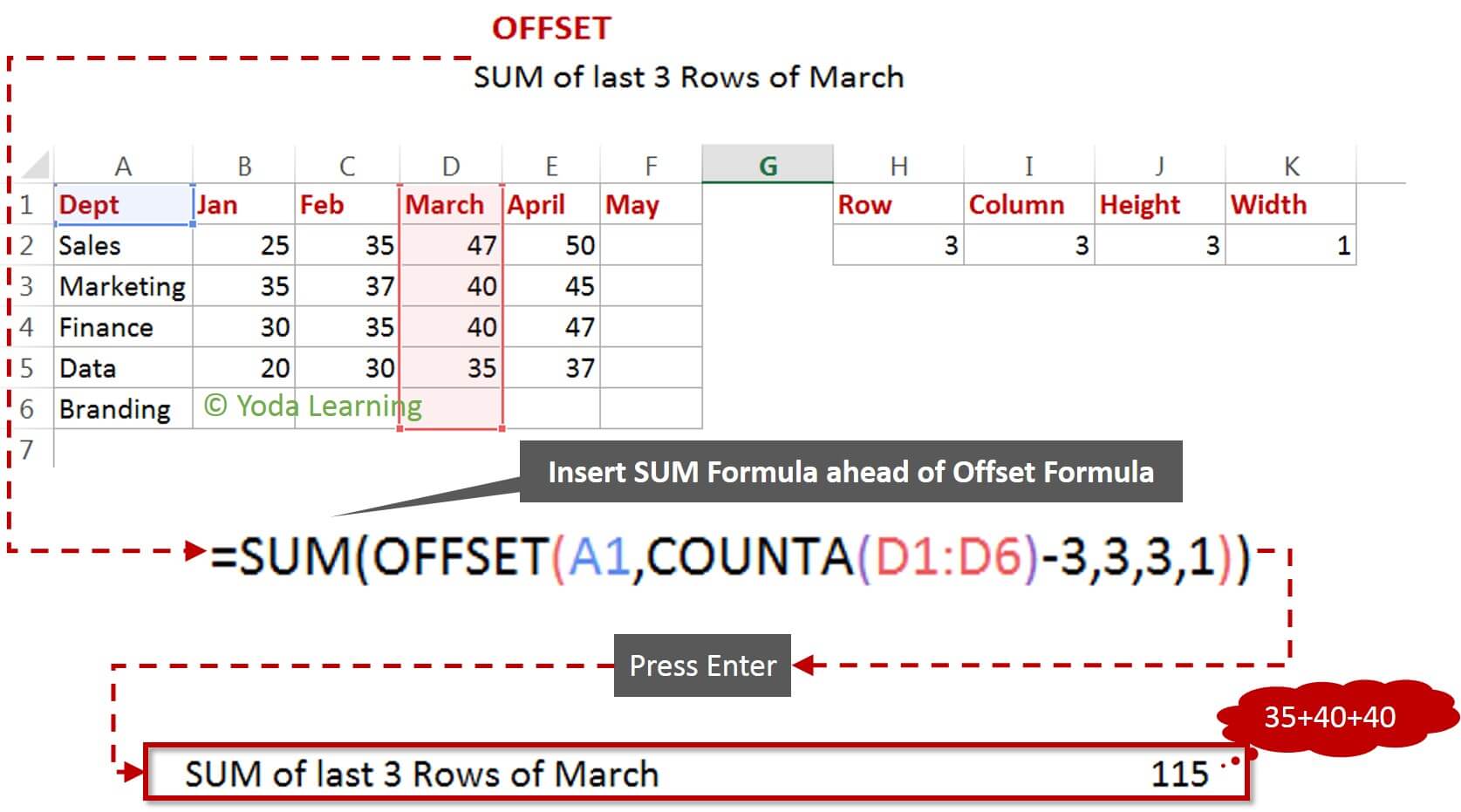
The OFFSET function is another powerful tool for dynamically referencing Excel table columns. This function returns a range that is offset from a specified range.

To dynamically reference a column using the OFFSET function, you can use the following formula:

=OFFSET(Sales, 0, MATCH("Region", Sales[#Headers], 0) - 1)

In this formula, the OFFSET function returns the entire column, offset by the relative position of the Region column within the table headers.

Leveraging the XLOOKUP function

The XLOOKUP function is a newer function in Excel that allows you to dynamically reference a value within a range. This function is similar to the VLOOKUP function but more powerful and flexible.

To dynamically reference a column using the XLOOKUP function, you can use the following formula:

=XLOOKUP("Region", Sales[#Headers], Sales)

In this formula, the XLOOKUP function returns the entire column, matching the Region column within the table headers.

Creating dynamic named ranges

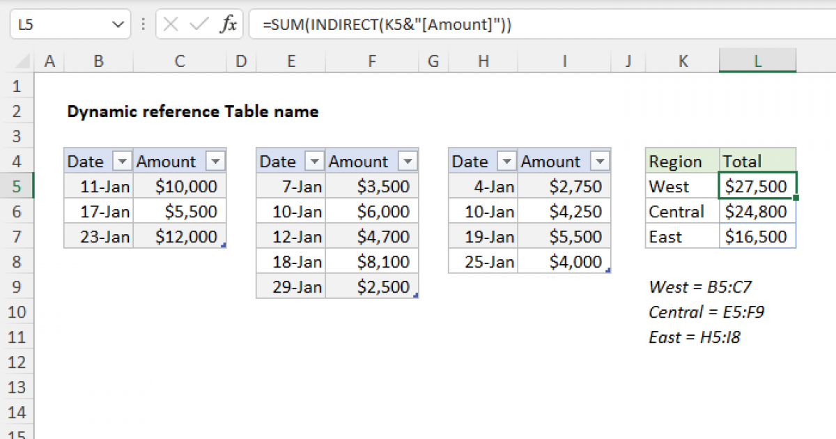
Another way to dynamically reference an Excel table column is by creating a dynamic named range. A dynamic named range is a range that is defined using a formula, allowing you to reference the range dynamically.

To create a dynamic named range, you can use the following formula:

=Sales[Region]

In this formula, the Sales[Region] notation creates a dynamic named range that references the Region column within the Sales table.

Gallery of Excel Column Reference Methods

Frequently Asked Questions

What is the difference between the `Tabela` notation and the `INDEX` and `MATCH` functions?

The `Tabela` notation is a simpler and more readable way to reference a column within a table, while the `INDEX` and `MATCH` functions provide more flexibility and power.

Can I use the `XLOOKUP` function to reference a column in a table?

Yes, you can use the `XLOOKUP` function to reference a column in a table. This function is more powerful and flexible than the `VLOOKUP` function.

How do I create a dynamic named range in Excel?

To create a dynamic named range in Excel, you can use a formula that references the column within the table. For example, `=Sales[Region]` creates a dynamic named range that references the `Region` column within the `Sales` table.

In conclusion, dynamically referencing columns in an Excel table can save you time and reduce errors. Whether you use the Tabela notation, the INDEX and MATCH functions, the OFFSET function, the XLOOKUP function, or create a dynamic named range, there are several ways to achieve this. By mastering these methods, you can take your data analysis to the next level and become more productive in Excel.