5 Ways To Aggregate Excel Row Data Easily

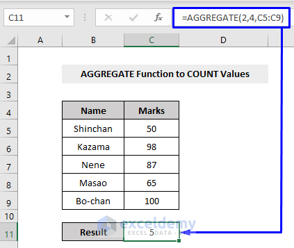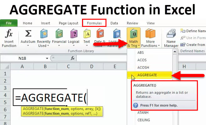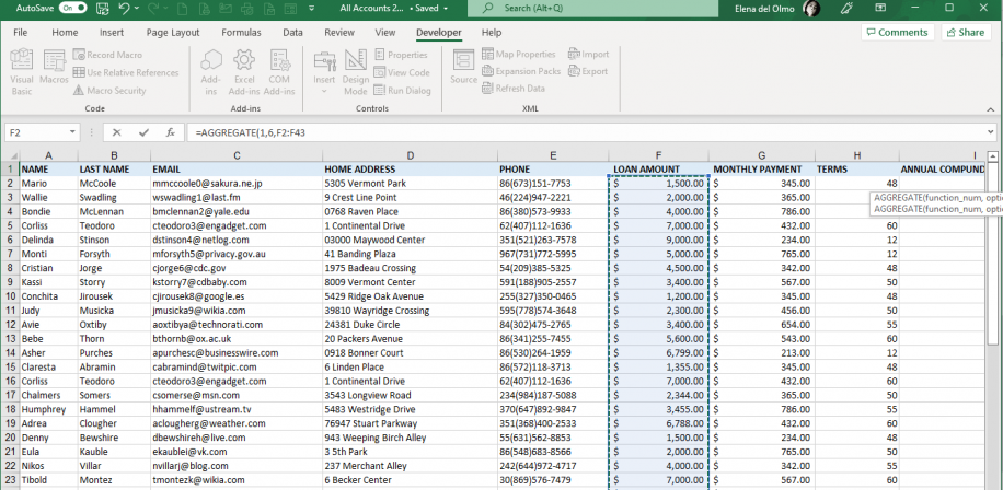
Data aggregation is a fundamental concept in data analysis, and Excel provides several methods to accomplish this task. Aggregating data involves collecting and summarizing data from multiple rows or columns to gain insights and make informed decisions. In this article, we will discuss five ways to aggregate Excel row data easily.

Working with large datasets can be overwhelming, and summarizing data is crucial to identify trends, patterns, and correlations. Excel offers various functions and features to aggregate data, including formulas, pivot tables, and Power Query. These tools enable users to extract meaningful information from their data, making it easier to analyze and visualize.

Whether you are a business professional, data analyst, or simply someone who works with data, this article will provide you with the skills to aggregate Excel row data efficiently. By mastering these techniques, you will be able to extract insights from your data and make better decisions.

Method 1: Using the SUMIF Function

The SUMIF function is a popular choice for aggregating data in Excel. This function allows you to sum values in a specific column based on criteria you specify. To use the SUMIF function, follow these steps:

1. Select the cell where you want to display the aggregated data.
2. Type "=SUMIF(" and select the range of cells you want to sum.
3. Specify the criteria range and criteria.
4. Close the parentheses and press Enter.

For example, suppose you have a dataset with sales data, and you want to sum the sales for a specific region. You can use the SUMIF function to achieve this.

Method 2: Using Pivot Tables

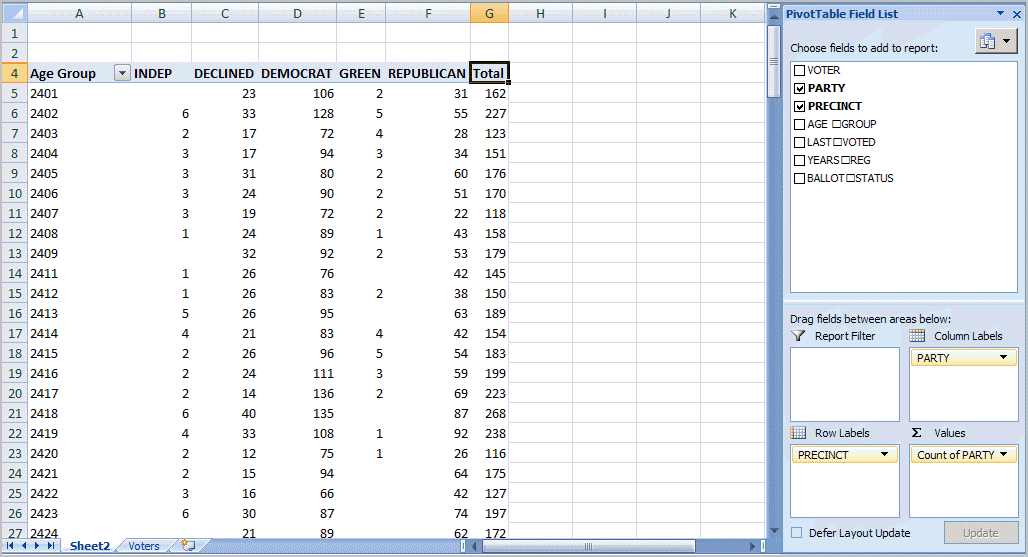
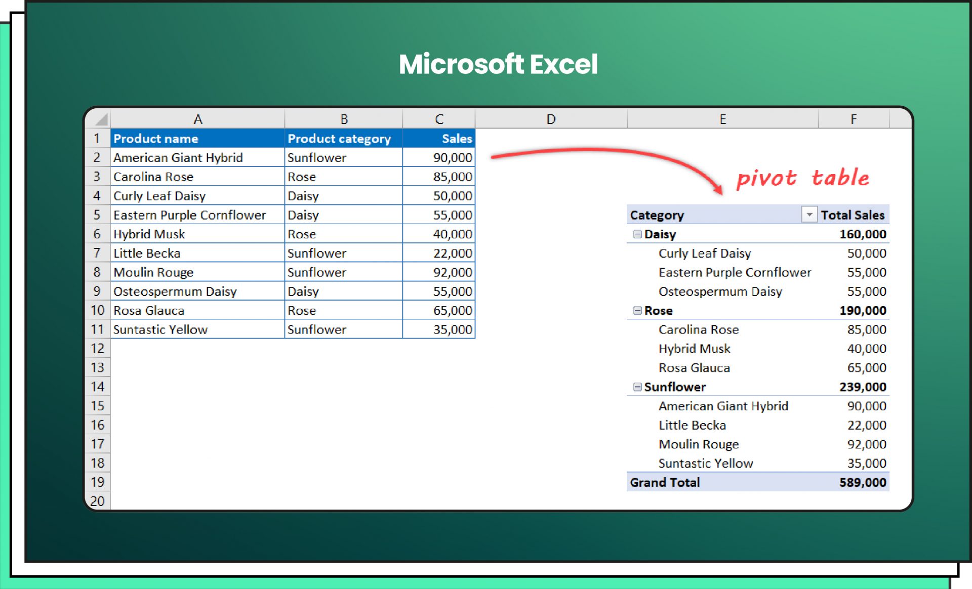
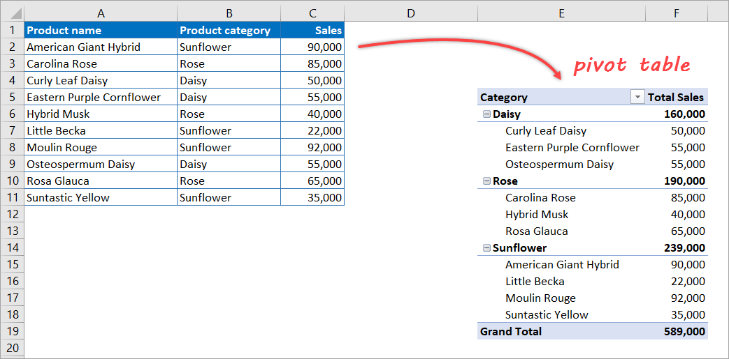
Pivot tables are a powerful tool for aggregating data in Excel. They allow you to summarize data from a large dataset and display the results in a concise and organized manner. To create a pivot table, follow these steps:

1. Select the cell range you want to analyze.
2. Go to the "Insert" tab and click on "PivotTable."
3. Choose a cell to place the pivot table.
4. Drag the fields you want to analyze to the "Rows" and "Columns" areas.
5. Right-click on the field and select "Summarize by" to choose the aggregation method.

For example, suppose you have a dataset with customer data, and you want to summarize the sales by region and product. You can use a pivot table to achieve this.

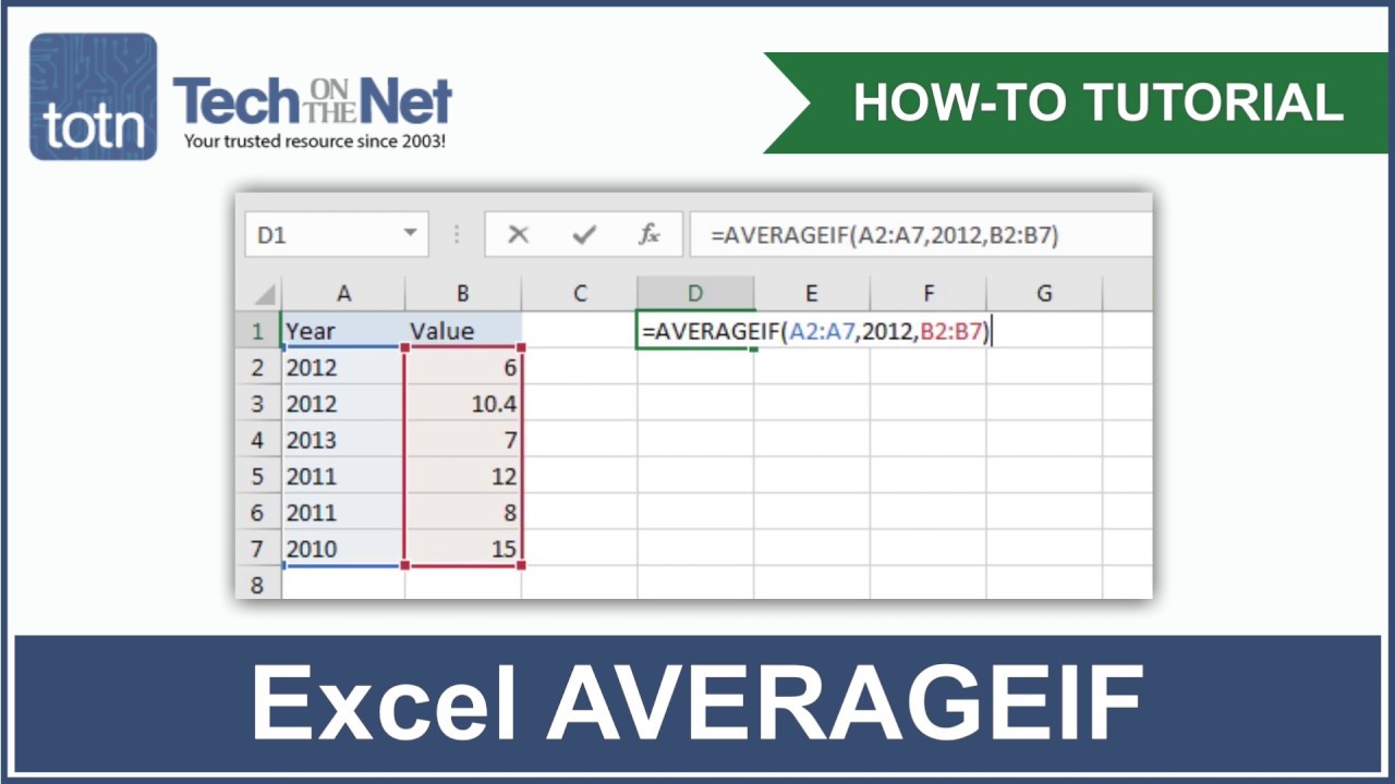
Method 3: Using the AVERAGEIF Function

The AVERAGEIF function is similar to the SUMIF function, but it calculates the average of a range of cells based on criteria you specify. To use the AVERAGEIF function, follow these steps:

1. Select the cell where you want to display the aggregated data.
2. Type "=AVERAGEIF(" and select the range of cells you want to average.
3. Specify the criteria range and criteria.
4. Close the parentheses and press Enter.

For example, suppose you have a dataset with exam scores, and you want to calculate the average score for a specific subject. You can use the AVERAGEIF function to achieve this.

Method 4: Using Power Query

Power Query is a powerful tool in Excel that allows you to aggregate data from multiple tables and data sources. To use Power Query, follow these steps:

1. Go to the "Data" tab and click on "From Table/Range."
2. Select the table or range you want to aggregate.
3. Click on "Group By" and select the columns you want to group by.
4. Choose the aggregation method and click "OK."

For example, suppose you have a dataset with sales data, and you want to aggregate the sales by region and product. You can use Power Query to achieve this.

Method 5: Using the SUBTOTAL Function

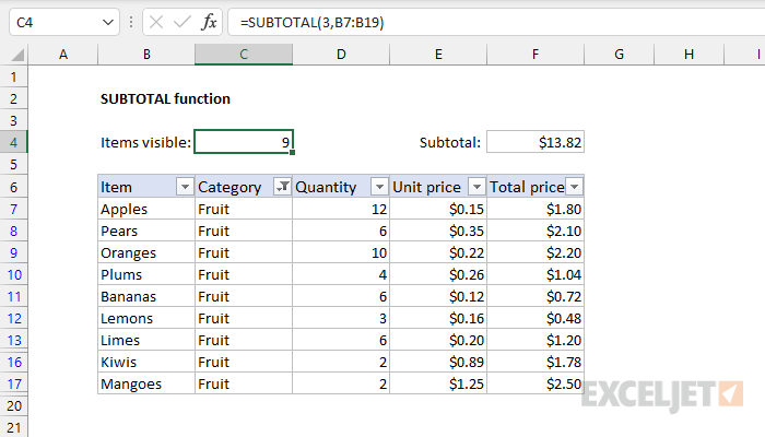
The SUBTOTAL function is a useful tool for aggregating data in Excel. It allows you to sum, average, or count a range of cells based on a criteria you specify. To use the SUBTOTAL function, follow these steps:

1. Select the cell where you want to display the aggregated data.
2. Type "=SUBTOTAL(" and select the function number you want to use.
3. Specify the range of cells you want to aggregate.
4. Close the parentheses and press Enter.

For example, suppose you have a dataset with sales data, and you want to sum the sales for a specific region. You can use the SUBTOTAL function to achieve this.

By mastering these five methods, you can easily aggregate Excel row data and gain insights from your data. Whether you are a business professional, data analyst, or simply someone who works with data, these techniques will help you to make better decisions and achieve your goals.

Gallery of Excel Data Aggregation

Frequently Asked Questions

By following these methods and tips, you can easily aggregate Excel row data and gain insights from your data. Remember to practice and experiment with different methods to find the one that works best for you.

Gallery of 5 Ways To Aggregate Excel Row Data Easily