5 Ways To Display Negative Numbers In Red In Excel

Negative numbers can be a crucial aspect of financial and numerical data, and being able to display them in a way that stands out is essential for clear and effective communication. In Excel, one of the most popular methods for highlighting negative numbers is to display them in red. This simple visual cue can greatly enhance the readability and understandability of your spreadsheets, making it easier for users to quickly identify and focus on the data that matters most.

Why Display Negative Numbers in Red?

Displaying negative numbers in red is a common practice in financial and numerical analysis. It serves several purposes:

• Visual distinction: Red negative numbers create a clear visual distinction from positive numbers, making it easier to scan and understand the data.
• Attention-grabbing: Red is a color that grabs attention, and using it for negative numbers helps draw the user's eye to areas of the spreadsheet that may require attention or action.
• Quick identification: By displaying negative numbers in red, users can quickly identify potential issues or areas of concern, such as losses, debts, or declines.

Method 1: Using Conditional Formatting

One of the most straightforward ways to display negative numbers in red is by using Excel's built-in Conditional Formatting feature.

Here's how to do it:

1. Select the range of cells you want to apply the formatting to.
2. Go to the Home tab in the Excel ribbon.
3. Click on the Conditional Formatting button in the Styles group.
4. Choose "New Rule" from the dropdown menu.
5. In the "New Formatting Rule" dialog box, select "Use a formula to determine which cells to format."
6. Enter the formula =A1<0, assuming the active cell is A1.
7. Click on the Format button and select a red font color.
8. Click OK to apply the rule.

Method 2: Using Number Formatting

Another way to display negative numbers in red is by using a custom number format.

Here's how to do it:

1. Select the range of cells you want to apply the formatting to.
2. Right-click on the selected cells and choose "Format Cells" from the context menu.
3. In the Format Cells dialog box, click on the Number tab.
4. Select "Custom" from the Category list.
5. In the Type field, enter the following format code: #,##0.00;[Red]-#,##0.00;
6. Click OK to apply the format.

Method 3: Using VBA Macro

If you prefer a more automated approach, you can use a VBA macro to display negative numbers in red.

Here's an example macro code:

Sub FormatNegativeNumbers()
    Dim cell As Range
    For Each cell In Selection
        If cell.Value < 0 Then
            cell.Font.Color = vbRed
        End If
    Next cell
End Sub

To use this macro, follow these steps:

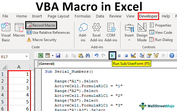
1. Open the Visual Basic Editor by pressing Alt + F11 or navigating to Developer > Visual Basic in the ribbon.
2. In the Visual Basic Editor, insert a new module by clicking Insert > Module.
3. Paste the macro code into the module.
4. Save the module by clicking File > Save.
5. To run the macro, select the range of cells you want to apply the formatting to and press Alt + F8 to open the Macro dialog box.
6. Select the "FormatNegativeNumbers" macro and click Run.

Method 4: Using Excel Add-ins

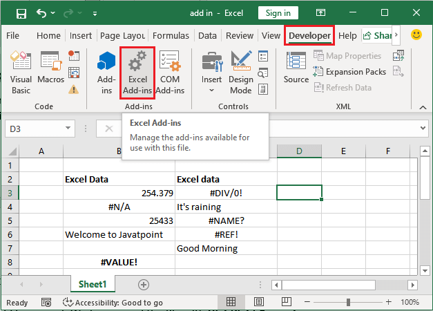
There are several Excel add-ins available that can help you display negative numbers in red.

Some popular add-ins include:

• Power Query
• Power Pivot
• ASAP Utilities

These add-ins often provide a range of formatting options, including the ability to display negative numbers in red.

Method 5: Using Excel Templates

Finally, you can use Excel templates to display negative numbers in red.

Many Excel templates, such as the built-in "Accounting" template, include pre-defined formatting rules that display negative numbers in red.

By using one of these methods, you can easily display negative numbers in red in your Excel spreadsheets, making it easier to analyze and understand your data.

Gallery of Excel Negative Number Formatting