Excel Formula For Last Month Data

Effective data analysis in Excel often requires working with dates and filtering data based on specific time frames, such as the previous month. Excel provides several formulas and functions that can help you extract data for the last month, depending on the current date. Below are some methods to achieve this, assuming your data is organized in a table with dates in one column and corresponding data in another.

1. Using the `TODAY()` Function

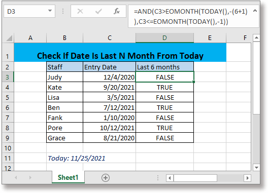
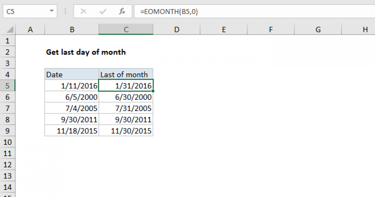
The TODAY() function returns the current date. You can use it in conjunction with the EOMONTH function to find the last date of the previous month and then filter your data accordingly.

Formula to Find the Last Date of the Previous Month:

=EOMONTH(TODAY(),-1)

This formula takes the current date and moves back one month, then returns the last day of that month.

Using `EOMONTH` and `TODAY()` to Filter Data:

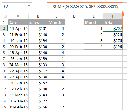
Assuming your dates are in column A and the data you want to sum or analyze is in column B, you can use the following formula to sum data for the last month:

=SUMIFS(B:B, A:A, ">="&EOMONTH(TODAY(),-1)-DAY(EOMONTH(TODAY(),-1))+1, A:A, "<="&EOMONTH(TODAY(),-1))

This formula calculates the sum of values in column B for dates in column A that fall within the last month.

2. Using the `DATEDIF` Function

Another approach is using the DATEDIF function, which calculates the difference between two dates in a specified interval (days, months, years). However, this function is not as straightforward for filtering data but can be useful for calculating periods.

3. Using Power Query

For more complex data analysis and dynamic date filtering, Power Query (available in Excel 2010 and later versions) is a powerful tool. You can load your data into Power Query, apply filters based on dynamic dates (such as the previous month), and then load the filtered data back into your Excel worksheet.

Step to load data into Power Query:
- Go to Data > From Table/Range
- Select your data range and click OK
Filtering Data for the Last Month in Power Query:
- In the Power Query Editor, click Add Column
- Use the Date function to create a filter, for example: = Date.Year([Date]) = Date.Year(Date.AddMonths(Date.From(DateTime.LocalNow()), -1)) and Date.Month([Date]) = Date.Month(Date.AddMonths(Date.From(DateTime.LocalNow()), -1))
- Then, filter your table based on this new column.

4. Using VBA Macros

If you're comfortable with VBA, you can also create a macro that automates the process of filtering data for the last month. This approach can be more complex but offers high customization flexibility.

Example VBA Macro

Sub FilterLastMonth()
    Dim ws As Worksheet
    Set ws = ThisWorkbook.Sheets("YourSheetName")
    
    Dim lastMonth As Date
    lastMonth = DateAdd("m", -1, Date)
    
    ws.AutoFilterMode = False
    ws.Range("A1").AutoFilter Field:=1, Criteria1:= _
        ">=" & CLng(lastMonth), Operator:=xlAnd, Criteria2:="<=" & CLng(Date)
    
    ' Further actions or filters as needed
End Sub

Replace "YourSheetName" with the name of the sheet containing your data.

Conclusion

Choosing the right method depends on your specific needs, the version of Excel you're using, and your comfort level with formulas, Power Query, or VBA. Each approach has its advantages, and combining them can lead to powerful data analysis capabilities.