Mastering Excel Conditional Formatting For Dates

Excel is an incredibly powerful tool for data analysis, and one of its most useful features is conditional formatting. This feature allows you to highlight cells based on specific conditions, making it easier to spot trends, patterns, and outliers in your data. When it comes to working with dates in Excel, conditional formatting can be particularly useful. In this article, we'll explore how to master Excel conditional formatting for dates, including how to highlight specific date ranges, create custom formatting rules, and use formulas to format dates.

The Importance of Date Formatting in Excel

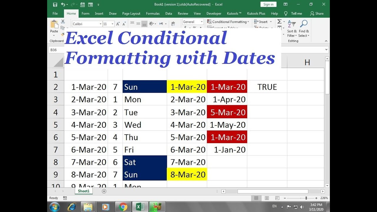
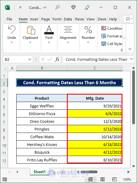
Dates are a crucial aspect of many datasets, and being able to format them effectively can make a huge difference in how easily you can analyze and understand your data. Conditional formatting can help you highlight important dates, such as deadlines, anniversaries, or birthdays, making it easier to focus on the most critical information.

How to Apply Basic Conditional Formatting to Dates

Before we dive into more advanced techniques, let's cover the basics of applying conditional formatting to dates in Excel. To get started, follow these steps:

Select the cells that contain the dates you want to format.
Go to the Home tab in the Excel ribbon.
Click on the Conditional Formatting button in the Styles group.
Select "Highlight Cells Rules" from the drop-down menu.
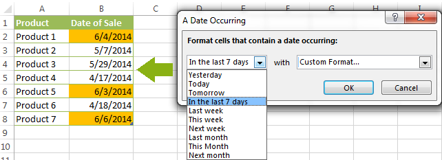
Choose "A Date Occurring" from the submenu.

This will open the Conditional Formatting Rules Manager dialog box, where you can specify the formatting rules you want to apply.

Creating Custom Formatting Rules for Dates

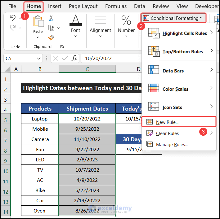
While the basic formatting rules in Excel are useful, you may need to create custom rules to suit your specific needs. To create a custom formatting rule for dates, follow these steps:

Select the cells that contain the dates you want to format.
Go to the Home tab in the Excel ribbon.
Click on the Conditional Formatting button in the Styles group.
Select "New Rule" from the drop-down menu.
Choose "Use a formula to determine which cells to format" from the submenu.

This will open the Format Values Where This Formula is True dialog box, where you can enter a formula to specify the formatting rule.

Using Formulas to Format Dates

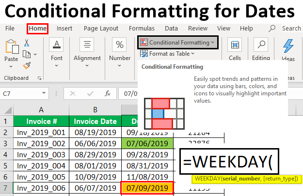
Formulas are a powerful way to format dates in Excel, allowing you to create complex formatting rules that meet your specific needs. Here are a few examples of formulas you can use to format dates:

=TODAY() - Highlights cells that contain today's date.
=A1>TODAY() - Highlights cells that contain dates later than today.
=A1<TODAY() - Highlights cells that contain dates earlier than today.
=WEEKNUM(A1, 2)>20 - Highlights cells that contain dates that fall in the last week of the year.

Advanced Techniques for Formatting Dates

Once you've mastered the basics of conditional formatting for dates, you can explore more advanced techniques to take your formatting to the next level. Here are a few examples:

Highlighting specific date ranges: Use the DATEDIF function to highlight cells that contain dates within a specific range.
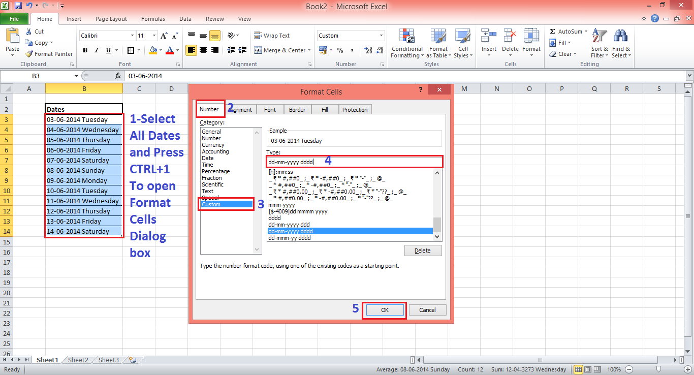
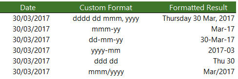
Creating custom date formats: Use the TEXT function to create custom date formats that meet your specific needs.
Using multiple formatting rules: Use the Conditional Formatting Rules Manager dialog box to create multiple formatting rules that apply to the same range of cells.

Best Practices for Formatting Dates in Excel

When formatting dates in Excel, there are a few best practices to keep in mind:

Use clear and consistent formatting: Use a consistent formatting style throughout your workbook to make it easier to understand and analyze your data.
Use meaningful formatting rules: Use formatting rules that are meaningful and relevant to your data, rather than simply applying formatting for the sake of it.
Test your formatting rules: Test your formatting rules thoroughly to ensure they are working as intended.

Conclusion

Mastering Excel conditional formatting for dates is a powerful way to enhance your data analysis and visualization skills. By applying basic formatting rules, creating custom formatting rules, and using formulas to format dates, you can take your Excel skills to the next level. Remember to follow best practices for formatting dates, and don't be afraid to experiment and try new things. With practice and patience, you'll become a master of Excel conditional formatting for dates.

Gallery of Excel Date Formatting

FAQs

What is conditional formatting in Excel?

Conditional formatting is a feature in Excel that allows you to highlight cells based on specific conditions, such as dates, numbers, or text.

How do I apply basic conditional formatting to dates in Excel?

To apply basic conditional formatting to dates in Excel, select the cells that contain the dates, go to the Home tab, click on the Conditional Formatting button, and select "Highlight Cells Rules" from the drop-down menu.

How do I create a custom formatting rule for dates in Excel?

To create a custom formatting rule for dates in Excel, select the cells that contain the dates, go to the Home tab, click on the Conditional Formatting button, and select "New Rule" from the drop-down menu. Then, choose "Use a formula to determine which cells to format" from the submenu.