Google Sheets is a powerful tool that offers a wide range of functions to help users manage and analyze data efficiently. One of the most useful functions in Google Sheets is the CHOOSE function. The CHOOSE function allows users to select a value from a list of options based on a specified index number. In this article, we will explore five ways to use the CHOOSE function in Google Sheets.
The CHOOSE function is a versatile function that can be used in various scenarios, from simple data analysis to complex data manipulation. By mastering the CHOOSE function, users can streamline their workflow, reduce errors, and make data-driven decisions with confidence. Whether you're a beginner or an advanced user, this article will provide you with practical examples and expert tips on how to use the CHOOSE function in Google Sheets.
What is the CHOOSE Function in Google Sheets?
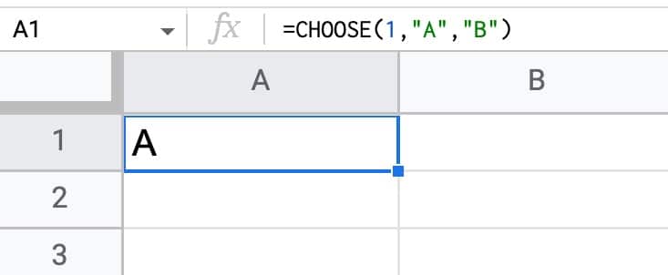
The CHOOSE function in Google Sheets is a lookup function that returns a value from a list of options based on a specified index number. The syntax of the CHOOSE function is:
CHOOSE(index, option1, [option2],...)
- index: The index number of the value to be returned. This can be a number, a cell reference, or a formula that returns a number.
- option1: The first option in the list.
- [option2]: The second option in the list (optional). *...: Additional options in the list (optional).
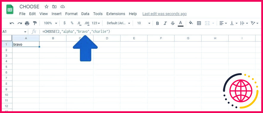
For example, if you want to return the value "Apple" from a list of fruits based on the index number 2, you can use the following formula:
CHOOSE(2, "Banana", "Apple", "Orange")
This formula will return the value "Apple" because it is the second option in the list.

1. Using the CHOOSE Function to Return a Value from a List
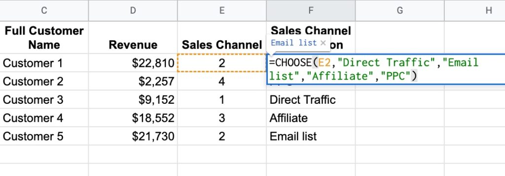
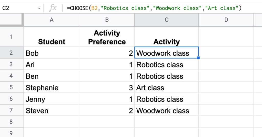
One of the simplest ways to use the CHOOSE function is to return a value from a list of options. For example, suppose you have a list of colors in cells A1:A5 and you want to return the color based on the index number in cell B1.
| Index | Color |
|---|---|
| 1 | Red |
| 2 | Blue |
| 3 | Green |
| 4 | Yellow |
| 5 | Purple |
To return the color based on the index number, you can use the following formula:
CHOOSE(B1, "Red", "Blue", "Green", "Yellow", "Purple")
Assuming the index number in cell B1 is 3, this formula will return the value "Green".
Practical Example:
Suppose you have a list of employee names in cells A1:A10 and you want to return the name based on the index number in cell B1. You can use the following formula:
CHOOSE(B1, "John", "Mary", "David", "Emily", "Michael", "Sarah", "Kevin", "Olivia", "William")
Assuming the index number in cell B1 is 5, this formula will return the value "Michael".

2. Using the CHOOSE Function with Multiple Criteria
The CHOOSE function can also be used with multiple criteria to return a value from a list of options. For example, suppose you have a list of products in cells A1:A10 and you want to return the product based on the index number in cell B1 and the category in cell C1.
| Index | Product | Category |
|---|---|---|
| 1 | Phone | Electronics |
| 2 | Laptop | Electronics |
| 3 | Tablet | Electronics |
| 4 | Chair | Furniture |
| 5 | Desk | Furniture |
| 6 | Book | Books |
| 7 | Pen | Stationery |
| 8 | Paper | Stationery |
| 9 | Bag | Accessories |
| 10 | Watch | Accessories |
To return the product based on the index number and category, you can use the following formula:
CHOOSE(B1, IF(C1="Electronics", "Phone", IF(C1="Furniture", "Chair", IF(C1="Books", "Book", IF(C1="Stationery", "Pen", IF(C1="Accessories", "Bag", "Unknown"))))))
Assuming the index number in cell B1 is 2 and the category in cell C1 is "Electronics", this formula will return the value "Laptop".
Practical Example:
Suppose you have a list of student grades in cells A1:A10 and you want to return the grade based on the index number in cell B1 and the subject in cell C1. You can use the following formula:
CHOOSE(B1, IF(C1="Math", "A", IF(C1="Science", "B", IF(C1="English", "C", IF(C1="History", "D", IF(C1="Geography", "E", "Unknown"))))))
Assuming the index number in cell B1 is 3 and the subject in cell C1 is "English", this formula will return the value "C".

3. Using the CHOOSE Function with a Drop-Down List
The CHOOSE function can also be used with a drop-down list to return a value from a list of options. For example, suppose you have a drop-down list of countries in cell A1 and you want to return the capital based on the selected country.
| Country | Capital |
|---|---|
| USA | Washington |
| Canada | Ottawa |
| Mexico | Mexico City |
To return the capital based on the selected country, you can use the following formula:
CHOOSE(MATCH(A1, {"USA", "Canada", "Mexico"}, 0), "Washington", "Ottawa", "Mexico City")
Assuming the selected country in cell A1 is "Canada", this formula will return the value "Ottawa".
Practical Example:
Suppose you have a drop-down list of cities in cell A1 and you want to return the population based on the selected city.
| City | Population |
|---|---|
| New York | 8,420,527 |
| Los Angeles | 3,999,759 |
| Chicago | 2,670,504 |
You can use the following formula:
CHOOSE(MATCH(A1, {"New York", "Los Angeles", "Chicago"}, 0), 8420527, 3999759, 2670504)
Assuming the selected city in cell A1 is "Chicago", this formula will return the value 2670504.

4. Using the CHOOSE Function with a Nested IF Statement
The CHOOSE function can also be used with a nested IF statement to return a value from a list of options. For example, suppose you have a list of exam scores in cells A1:A10 and you want to return the grade based on the score.
| Score | Grade |
|---|---|
| 90-100 | A |
| 80-89 | B |
| 70-79 | C |
| 60-69 | D |
| 0-59 | F |
To return the grade based on the score, you can use the following formula:
CHOOSE(IF(A1>=90, 1, IF(A1>=80, 2, IF(A1>=70, 3, IF(A1>=60, 4, 5)))), "A", "B", "C", "D", "F")
Assuming the score in cell A1 is 85, this formula will return the value "B".
Practical Example:
Suppose you have a list of customer types in cells A1:A10 and you want to return the discount based on the type.
| Type | Discount |
|---|---|
| VIP | 10% |
| Premium | 5% |
| Basic | 0% |
You can use the following formula:
CHOOSE(IF(A1="VIP", 1, IF(A1="Premium", 2, 3)), 0.1, 0.05, 0)
Assuming the type in cell A1 is "Premium", this formula will return the value 0.05.

5. Using the CHOOSE Function with an Array Formula
The CHOOSE function can also be used with an array formula to return a value from a list of options. For example, suppose you have a list of stock prices in cells A1:A10 and you want to return the price based on the index number.
| Index | Price |
|---|---|
| 1 | 100 |
| 2 | 120 |
| 3 | 150 |
| 4 | 180 |
| 5 | 200 |
To return the price based on the index number, you can use the following formula:
=INDEX(CHOOSE(B1, 100, 120, 150, 180, 200), 0)
Assuming the index number in cell B1 is 3, this formula will return the value 150.
Practical Example:
Suppose you have a list of employee salaries in cells A1:A10 and you want to return the salary based on the index number.
| Index | Salary |
|---|---|
| 1 | 50000 |
| 2 | 60000 |
| 3 | 70000 |
| 4 | 80000 |
| 5 | 90000 |
You can use the following formula:
=INDEX(CHOOSE(B1, 50000, 60000, 70000, 80000, 90000), 0)
Assuming the index number in cell B1 is 4, this formula will return the value 80000.


What is the CHOOSE function in Google Sheets?
+The CHOOSE function in Google Sheets is a lookup function that returns a value from a list of options based on a specified index number.
How do I use the CHOOSE function in Google Sheets?
+The CHOOSE function can be used in various ways, including returning a value from a list of options, using multiple criteria, using a drop-down list, using a nested IF statement, and using an array formula.
What are some practical examples of using the CHOOSE function in Google Sheets?
+Some practical examples of using the CHOOSE function in Google Sheets include returning a value from a list of options, using multiple criteria, using a drop-down list, using a nested IF statement, and using an array formula.
We hope this article has helped you understand the CHOOSE function in Google Sheets and how to use it in various scenarios. Whether you're a beginner or an advanced user, the CHOOSE function is a powerful tool that can help you streamline your workflow and make data-driven decisions with confidence.


![How to Use CHOOSE Function in Google Sheets [Purpose and Examples]](https://infoinspired.com/wp-content/uploads/2017/12/Simple-Lookup-using-Match-Choose-Combination-250x110.jpg)

![How to Use CHOOSE Function in Google Sheets [Purpose and Examples]](https://infoinspired.com/wp-content/uploads/2017/12/Choose-Function-Examples-in-Google-Sheets-1.jpg)
:max_bytes(150000):strip_icc()/002_google-spreadsheet-functions-tutorial-4163591-4cb6b6c56ba645c8aee4f27893146267.jpg)
:max_bytes(150000):strip_icc()/001_google-spreadsheet-functions-tutorial-4163591-c3d77005d89942b5abfe1b19ce0e35f4.jpg)
![How to Use CHOOSE Function in Google Sheets [Purpose and Examples]](https://infoinspired.com/wp-content/uploads/2017/12/Choose-Vs-Switch-in-Google-Sheets-2.jpg)

